Statistical Modelling: Predicting

In this chapter you will learn:

how to use your statistical model to make a prediction

1 Predicting

One of the motivations we discussed motivations for statistical modelling was that models help us to make quantitative predictions about the system which we are studying.¹

Now that you have your best-specified model, you may want to use it to make a response prediction², e.g. “what would I expect the value of my response to be at a different value of my predictor?”

The predicting process outlined here is similar regardless of your model structure (e.g. error distribution assumption). You can use the same process for models of any structure.

1.1 The process

Here we will go through the steps involved in using your model to make a prediction about your response, including (most importantly):

Step Zero: consider your prediction limits

Before using your model to make a prediction, ask yourself: is it even logical to make this prediction?

Things you should consider:

do I have a numeric predictor in my best-specified model?

If you have only categorical predictors in your model, you can not use your model to make a prediction outside the categories already in your model.

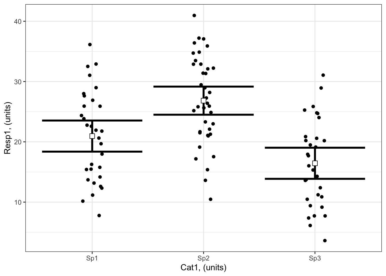
Let’s bring in our Example 1 from the last chapter on Reporting to illustrate the prediction limits of models with only categorical predictors:

Resp1 ~ Cat1

Here you can see the modelled Resp1 when Cat1 is Sp1, Sp2 or Sp3. You are not able to make a prediction for Cat1 = Sp4 or Cat1 = Sp63. This is limits of prediction limit when you have a categorical predictor. You are able to report the variability in Resp1 that is explained by Cat1 - this can give you an idea for how much Resp1 might vary if you study a new species.

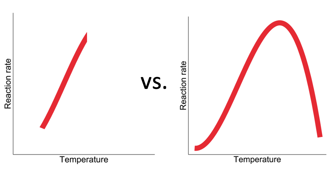
Can I assume that my model assumptions will hold under my prediction conditions?

By using your model to make a prediction, you are assuming that the same processes that govern the relationship(s) between your predictor(s) and response will hold at the new value of your predictor. For example, you might have used a linear shape assumption that was appropriate for modelling how growth varies due to temperature for your data, but now you want to estimate growth at an even higher temperature than you tested. Is this appropriate? Would it be possible that temperature has exceeded a tolerance limit and that growth starts to respond non-linearly with temperature?

As you can see, you need to consider prediction limits particularly when you are making a prediction using a value of your predictor outside the range of your predictor used to fit your model.

You also need to consider prediction limits when you are wanting to predict your response at a future time or different location.

In all cases: Think about the mechanisms underlying your hypothesis to consider if they are likely to be the same under your prediction conditions. This will help you decide if making a prediction is appropriate.

Step One: Define the predictor values for your response prediction

The first step in using your model to make a response prediction is to define the values of your predictor(s) at which you want to make the response prediction. Note that you need to define a value for each of the predictors in your model, the defined values need to be in a data frame, and the columns should be given the same names as your predictors.

Step Two: Make your response prediction

You can use the predict()³ function to predict the value of your response.

1.2 Examples

Note that Example 1 (Resp1 ~ Cat1) and Example 2 (Resp2 ~ Cat2 + Cat3 + Cat2:Cat3 + 1) from the previous chapter on Reporting only contained categorical predictors, so we will not explore them further here.

Examples 3 (Resp3 ~ Cont4 + 1) and 4 (Resp4 ~ Cat5 + Cont6 + Cat5:Cont6 + 1) each contain a numeric predictor, so we will use those here as an example of how to use your models to make a prediction of your response.

Example 3: Resp3 ~ Cont4 + 1

Here’s a reminder of Example 3 (Resp3 ~ Cont4 + 1):

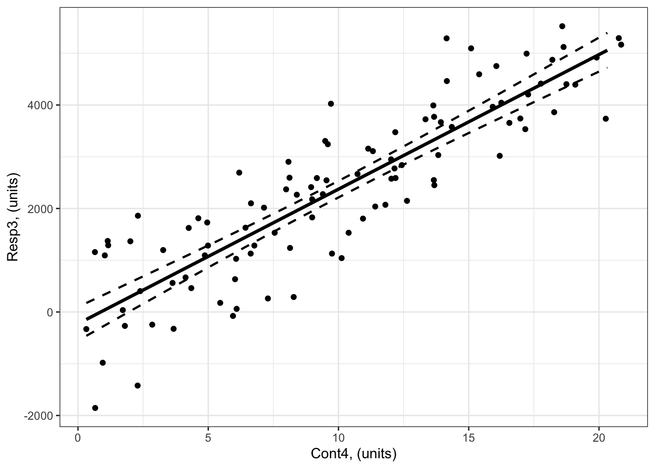
What is the predicted response of `Resp3` when `Cont4 = 30`?

## Step One: Define the predictor values for your response prediction
forPred <- data.frame(Cont4 = 30) # the values of my predictor at which I want a response prediction

## Step Two: Make your response prediction
myPred<-predict(bestMod3, # the model
                newdata = forPred, # the predictor values
                type = "link", # here, make the predictions on the link scale and we'll translate the back below
                se.fit = TRUE) # include uncertainty estimate

ilink <- family(bestMod3)$linkinv # get the conversion (inverse link) from the model to translate back to the response scale

### This can be added to our forPred data frame as:
forPred$Fit<-ilink(myPred$fit) # add your fit to the data frame
forPred$Lower<-ilink(myPred$fit - 1.96*myPred$se.fit) # add your uncertainty to the data frame, 95% confidence intervals
forPred$Upper<-ilink(myPred$fit + 1.96*myPred$se.fit) # add your uncertainty to the data frame, 95% confidence intervals


forPred

  Cont4      Fit    Lower    Upper
1    30 7574.809 6980.293 8169.325

Note that you get the response prediction in forPred$Fit = 7575 units and an estimate of uncertainty around this prediction as the 95% confidence intervals (6980 to 8169 units).

Note that you can also use the ggeffects package to make these predictions.

So the value of Resp3 when Cont4 = 30 units is 7575 units (95% confidence intervals: 6980 to 8169 units).

You can add this to your plot with:

# Set up your predictors for the visualized fit
forCont4<-seq(from = min(myDat3$Cont4), to = max(myDat3$Cont4), by = 1)# a sequence of numbers in your numeric predictor range
  
# create a data frame with your predictors
forVis<-expand.grid(Cont4 = forCont4) # expand.grid() function makes sure you have all combinations of predictors.  

# Get your model fit estimates at each value of your predictors
modFit<-predict(bestMod3, # the model
                newdata = forVis, # the predictor values
                type = "link", # here, make the predictions on the link scale and we'll translate the back below
                se.fit = TRUE) # include uncertainty estimate

ilink <- family(bestMod3)$linkinv # get the conversion (inverse link) from the model to translate back to the response scale

forVis$Fit<-ilink(modFit$fit) # add your fit to the data frame
forVis$Upper<-ilink(modFit$fit + 1.96*modFit$se.fit) # add your uncertainty to the data frame, 95% confidence intervals
forVis$Lower<-ilink(modFit$fit - 1.96*modFit$se.fit) # add your uncertainty to the data frame


library(ggplot2) # load ggplot2 library

ggplot() + # start ggplot
  
  geom_point(data = myDat3, # add observations to your plot
             mapping = aes(x = Cont4, y = Resp3)) + # control position of data points so they are easier to see on the plot
  
  geom_line(data = forVis, # add the modelled fit to your plot
              mapping = aes(x = Cont4, y = Fit),
              size = 1.2) + # control thickness of line
  
    geom_line(data = forVis, # add uncertainty to your plot (upper line)
              mapping = aes(x = Cont4, y = Upper),
              size = 0.8, # control thickness of line
              linetype = 2) + # control style of line
  
      geom_line(data = forVis, # add uncertainty to your plot (lower line)
              mapping = aes(x = Cont4, y = Lower),
              size = 0.8, # control thickness of line
              linetype = 2) + # control style of line
  
  ### NEW!  Adding your response prediction to the plot:
  geom_point(data = forPred, # prediction data frame
             mapping = aes(x = Cont4, y = Fit), # coordinates of prediction
             col = "red", # change point colour
             size = 3) + # change point size
  
  ### NEW!  Adding errorbars for your response prediction to the plot:
  geom_errorbar(data = forPred, # prediction data frame
             mapping = aes(x = Cont4, ymax = Upper, ymin = Lower), # coordinates of prediction
             width = 1, # the width of the error bars
             col = "red") + # change point colour
  
  
  ylab("Resp3, (units)") + # change y-axis label
  
  xlab("Cont4, (units)") + # change x-axis label
  
  theme_bw() # change ggplot theme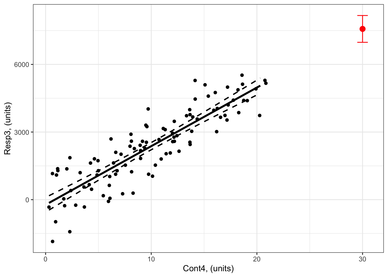

What are the predicted responses of `Resp3` when `Cont4 = 9` and `Cont4 = 22`?

## Step One: Define the predictor values for your response prediction
forPred <- data.frame(Cont4 = c(9,22)) # the values of my predictor at which I want a response prediction

## Step Two: Make your response prediction
myPred<-predict(bestMod3, # the model
                newdata = forPred, # the predictor values
                type = "link", # here, make the predictions on the link scale and we'll translate the back below
                se.fit = TRUE) # include uncertainty estimate

ilink <- family(bestMod3)$linkinv # get the conversion (inverse link) from the model to translate back to the response scale

### This can be added to our forPred data frame as:
forPred$Fit<-ilink(myPred$fit) # add your fit to the data frame
forPred$Lower<-ilink(myPred$fit - 1.96*myPred$se.fit) # add your uncertainty to the data frame, 95% confidence intervals
forPred$Upper<-ilink(myPred$fit + 1.96*myPred$se.fit) # add your uncertainty to the data frame, 95% confidence intervals


forPred

  Cont4      Fit    Lower    Upper
1     9 2113.604 1951.820 2275.387
2    22 5494.350 5114.867 5873.832

Note that you now get two predictions, one for Cont4 = 9 and one for Cont4 = 22:

The value of Resp3 when Cont4 = 9 units is 2114 units (95% confidence intervals: 1952 to 2275 units).
The value of Resp3 when Cont4 = 22 units is 5494 units (95% confidence intervals: 5115 to 5874 units).

You can add this to your plot with:

# Set up your predictors for the visualized fit
forCont4<-seq(from = min(myDat3$Cont4), to = max(myDat3$Cont4), by = 1)# a sequence of numbers in your numeric predictor range
  
# create a data frame with your predictors
forVis<-expand.grid(Cont4 = forCont4) # expand.grid() function makes sure you have all combinations of predictors.  

# Get your model fit estimates at each value of your predictors
modFit<-predict(bestMod3, # the model
                newdata = forVis, # the predictor values
                type = "link", # here, make the predictions on the link scale and we'll translate the back below
                se.fit = TRUE) # include uncertainty estimate

ilink <- family(bestMod3)$linkinv # get the conversion (inverse link) from the model to translate back to the response scale

forVis$Fit<-ilink(modFit$fit) # add your fit to the data frame
forVis$Upper<-ilink(modFit$fit + 1.96*modFit$se.fit) # add your uncertainty to the data frame, 95% confidence intervals
forVis$Lower<-ilink(modFit$fit - 1.96*modFit$se.fit) # add your uncertainty to the data frame


library(ggplot2) # load ggplot2 library

ggplot() + # start ggplot
  
  geom_point(data = myDat3, # add observations to your plot
             mapping = aes(x = Cont4, y = Resp3)) + # control position of data points so they are easier to see on the plot
  
  geom_line(data = forVis, # add the modelled fit to your plot
              mapping = aes(x = Cont4, y = Fit),
              size = 1.2) + # control thickness of line
  
    geom_line(data = forVis, # add uncertainty to your plot (upper line)
              mapping = aes(x = Cont4, y = Upper),
              size = 0.8, # control thickness of line
              linetype = 2) + # control style of line
  
      geom_line(data = forVis, # add uncertainty to your plot (lower line)
              mapping = aes(x = Cont4, y = Lower),
              size = 0.8, # control thickness of line
              linetype = 2) + # control style of line
  
  ### NEW!  Adding your response prediction to the plot:
  geom_point(data = forPred, # prediction data frame
             mapping = aes(x = Cont4, y = Fit), # coordinates of prediction
             col = "orange", # change point colour
             size = 3) + # change point size
  
  ### NEW!  Adding errorbars for your response prediction to the plot:
  geom_errorbar(data = forPred, # prediction data frame
             mapping = aes(x = Cont4, ymax = Upper, ymin = Lower), # coordinates of prediction
             width = 1, # the width of the error bars
             col = "orange") + # change point colour
  
  ylab("Resp3, (units)") + # change y-axis label
  
  xlab("Cont4, (units)") + # change x-axis label
  
  theme_bw() # change ggplot theme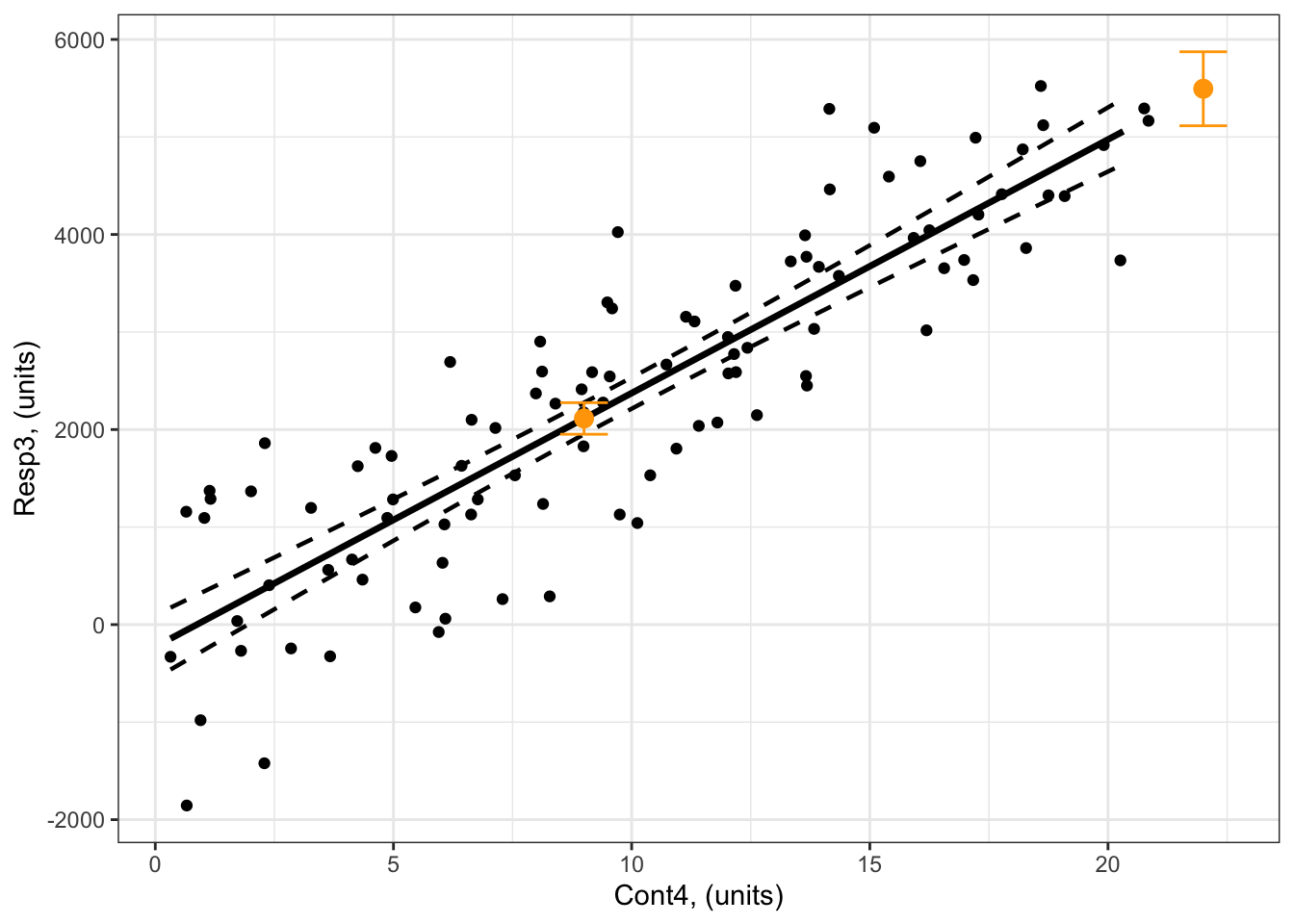

Example 4: Resp4 ~ Cat5 + Cont6 + Cat5:Cont6 + 1

Here’s a reminder of Example 4 (Resp4 ~ Cat5 + Cont6 + Cat5:Cont6 + 1):

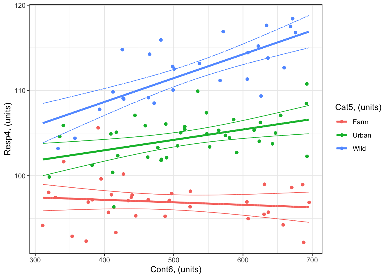
Example: What is the predicted response of `Resp4` when `Cont6 = 800` for `Cat5 = Urban`?

## Step One: Define the predictor values for your response prediction
forPred <- data.frame(Cont6 = 800,
                      Cat5 = "Urban") # the values of my predictor at which I want a response prediction

## Step Two: Make your response prediction
myPred<-predict(bestMod4, # the model
                newdata = forPred, # the predictor values
                type = "link", # here, make the predictions on the link scale and we'll translate the back below
                se.fit = TRUE) # include uncertainty estimate

ilink <- family(bestMod4)$linkinv # get the conversion (inverse link) from the model to translate back to the response scale

### This can be added to our forPred data frame as:
forPred$Fit<-ilink(myPred$fit) # add your fit to the data frame
forPred$Lower<-ilink(myPred$fit - 1.96*myPred$se.fit) # add your uncertainty to the data frame, 95% confidence intervals
forPred$Upper<-ilink(myPred$fit + 1.96*myPred$se.fit) # add your uncertainty to the data frame, 95% confidence intervals


forPred

  Cont6  Cat5      Fit    Lower    Upper
1   800 Urban 107.8597 105.4153 110.3041

So the value of Resp4 when Cont6 = 800 units for Cat5 = Urban is 107.9 units (95% confidence intervals: 105.4 to 110.3 units).

You can add this to your plot with:

#### i) choosing the values of your predictors at which to make a prediction
# Set up your predictors for the visualized fit
forCat5<-unique(myDat4$Cat5) # all levels of your categorical predictor
forCont6<-seq(from = min(myDat4$Cont6), to = max(myDat4$Cont6), by = 1)# a sequence of numbers in your numeric predictor range
  
# create a data frame with your predictors
forVis<-expand.grid(Cat5 = Cat5, Cont6 = forCont6) # expand.grid() function makes sure you have all combinations of predictors.  

#### ii) using `predict()` to use your model to estimate your response variable at those values of your predictor


# Get your model fit estimates at each value of your predictors
modFit<-predict(bestMod4, # the model
                newdata = forVis, # the predictor values
                type = "link", # here, make the predictions on the link scale and we'll translate the back below
                se.fit = TRUE) # include uncertainty estimate

ilink <- family(bestMod4)$linkinv # get the conversion (inverse link) from the model to translate back to the response scale

forVis$Fit<-ilink(modFit$fit) # add your fit to the data frame
forVis$Upper<-ilink(modFit$fit + 1.96*modFit$se.fit) # add your uncertainty to the data frame, 95% confidence intervals
forVis$Lower<-ilink(modFit$fit - 1.96*modFit$se.fit) # add your uncertainty to the data frame


#### iii) use the model estimates to plot your model fit


library(ggplot2) # load ggplot2 library

ggplot() + # start ggplot
  
  geom_point(data = myDat4, # add observations to your plot
             mapping = aes(x = Cont6, y = Resp4, col = Cat5)) + # control position of data points so they are easier to see on the plot
  
  geom_line(data = forVis, # add the modelled fit to your plot
              mapping = aes(x = Cont6, y = Fit, col = Cat5),
              size = 1.2) + # control thickness of line
  
    geom_line(data = forVis, # add uncertainty to your plot (upper line)
              mapping = aes(x = Cont6, y = Upper, col = Cat5),
              size = 0.4, # control thickness of line
              linetype = 2) + # control style of line
  
      geom_line(data = forVis, # add uncertainty to your plot (lower line)
              mapping = aes(x = Cont6, y = Lower, col = Cat5),
              size = 0.4, # control thickness of line
              linetype = 2) + # control style of line
  
  
    ### NEW!  Adding your response prediction to the plot:
  geom_point(data = forPred, # prediction data frame
             mapping = aes(x = Cont6, y = Fit, col = Cat5), # coordinates of prediction
             #col = "black", # change point colour
             size = 3) + # change point size
  
  ### NEW!  Adding errorbars for your response prediction to the plot:
  geom_errorbar(data = forPred, # prediction data frame
             mapping = aes(x = Cont6, ymax = Upper, ymin = Lower,  col = Cat5), # coordinates of prediction
             width = 20, # the width of the error bars
             #col = "black"
             ) + # change point colour
  
  ylab("Resp4, (units)") + # change y-axis label
  
  xlab("Cont6, (units)") + # change x-axis label
  
  labs(fill="Cat5, (units)", col="Cat5, (units)") + # change legend title
  
  theme_bw() # change ggplot theme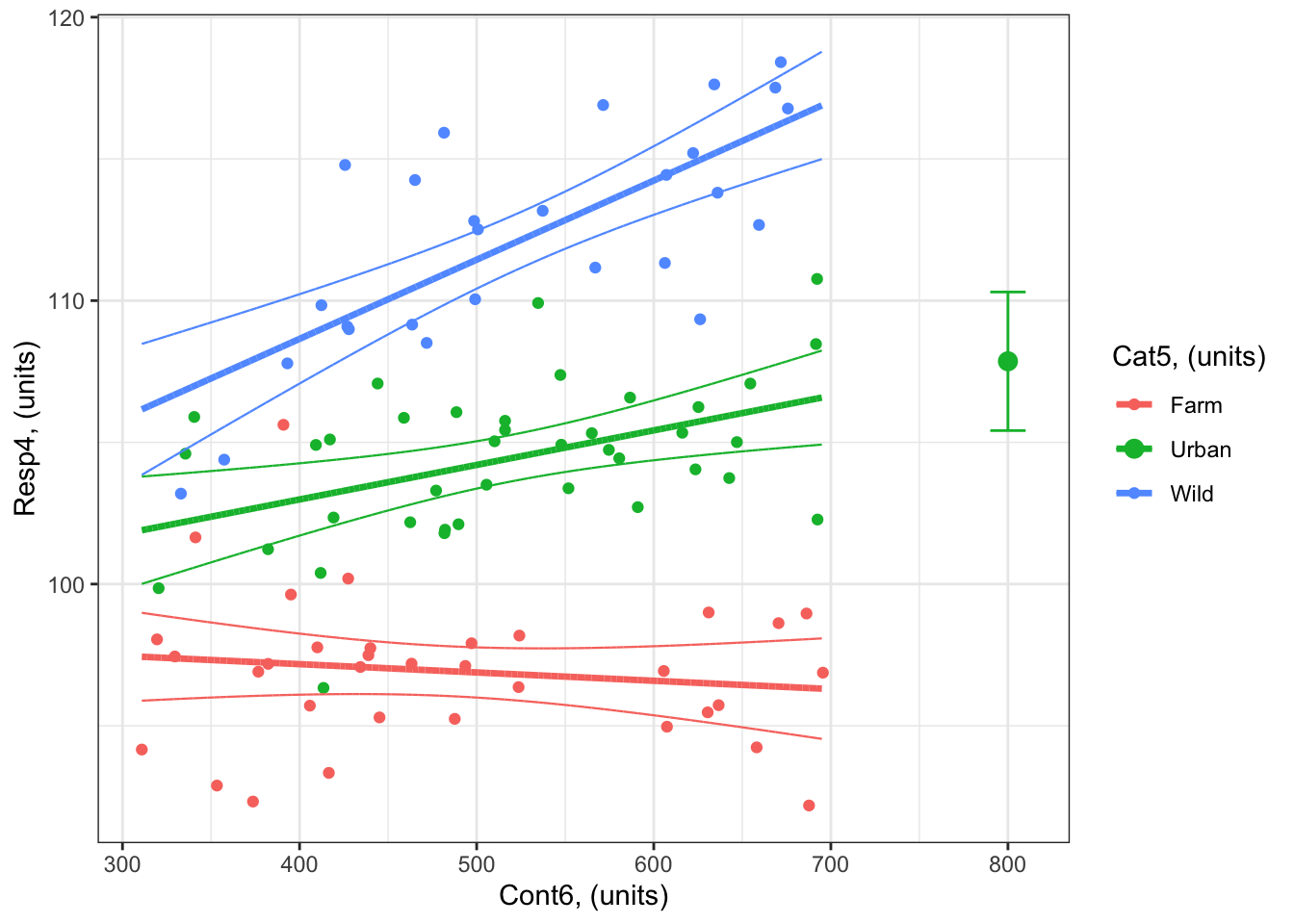

Example: What is the predicted response of `Resp4` when `Cont6 = 800` for both `Cat5 = Urban` and `Cat5 = Wild`?

Note the extra step with expand.grid() that allows you to quickly set up your predictor values for the prediction.

## Step One: Define the predictor values for your response prediction
forCat5 <- c("Urban", "Wild") # values of Cat5 for predictions
forCont6 <- 800 # value of Cont6 for prediction

forPred <- expand.grid(Cat5 = forCat5, Cont6 = forCont6) # expand.grid() function makes sure you have all combinations of predictors.

## Step Two: Make your response prediction
myPred<-predict(bestMod4, # the model
                newdata = forPred, # the predictor values
                type = "link", # here, make the predictions on the link scale and we'll translate the back below
                se.fit = TRUE) # include uncertainty estimate

ilink <- family(bestMod4)$linkinv # get the conversion (inverse link) from the model to translate back to the response scale

### This can be added to our forPred data frame as:
forPred$Fit<-ilink(myPred$fit) # add your fit to the data frame
forPred$Lower<-ilink(myPred$fit - 1.96*myPred$se.fit) # add your uncertainty to the data frame, 95% confidence intervals
forPred$Upper<-ilink(myPred$fit + 1.96*myPred$se.fit) # add your uncertainty to the data frame, 95% confidence intervals


forPred

   Cat5 Cont6      Fit    Lower    Upper
1 Urban   800 107.8597 105.4153 110.3041
2  Wild   800 119.8214 117.0121 122.6307

the value of Resp4 when Cont6 = 800 units is both Cat5 = Urban is 107.9 units (95% confidence intervals: 105.4 to 110.3 units).
the value of Resp4 when Cont6 = 800 units is both Cat5 = Wild is 119.8 units (95% confidence intervals: 117 to 122.6 units).

You can add this to your plot with:

#### i) choosing the values of your predictors at which to make a prediction
# Set up your predictors for the visualized fit
forCat5<-unique(myDat4$Cat5) # all levels of your categorical predictor
forCont6<-seq(from = min(myDat4$Cont6), to = max(myDat4$Cont6), by = 1)# a sequence of numbers in your numeric predictor range
  
# create a data frame with your predictors
forVis<-expand.grid(Cat5 = forCat5, Cont6 = forCont6) # expand.grid() function makes sure you have all combinations of predictors.  

#### ii) using `predict()` to use your model to estimate your response variable at those values of your predictor


# Get your model fit estimates at each value of your predictors
modFit<-predict(bestMod4, # the model
                newdata = forVis, # the predictor values
                type = "link", # here, make the predictions on the link scale and we'll translate the back below
                se.fit = TRUE) # include uncertainty estimate

ilink <- family(bestMod4)$linkinv # get the conversion (inverse link) from the model to translate back to the response scale

forVis$Fit<-ilink(modFit$fit) # add your fit to the data frame
forVis$Upper<-ilink(modFit$fit + 1.96*modFit$se.fit) # add your uncertainty to the data frame, 95% confidence intervals
forVis$Lower<-ilink(modFit$fit - 1.96*modFit$se.fit) # add your uncertainty to the data frame


#### iii) use the model estimates to plot your model fit


library(ggplot2) # load ggplot2 library

ggplot() + # start ggplot
  
  geom_point(data = myDat4, # add observations to your plot
             mapping = aes(x = Cont6, y = Resp4, col = Cat5)) + # control position of data points so they are easier to see on the plot
  
  geom_line(data = forVis, # add the modelled fit to your plot
              mapping = aes(x = Cont6, y = Fit, col = Cat5),
              size = 1.2) + # control thickness of line
  
    geom_line(data = forVis, # add uncertainty to your plot (upper line)
              mapping = aes(x = Cont6, y = Upper, col = Cat5),
              size = 0.4, # control thickness of line
              linetype = 2) + # control style of line
  
      geom_line(data = forVis, # add uncertainty to your plot (lower line)
              mapping = aes(x = Cont6, y = Lower, col = Cat5),
              size = 0.4, # control thickness of line
              linetype = 2) + # control style of line
  
  
    ### NEW!  Adding your response prediction to the plot:
  geom_point(data = forPred, # prediction data frame
             mapping = aes(x = Cont6, y = Fit, col = Cat5), # coordinates of prediction
             #col = "black", # change point colour
             size = 3) + # change point size
  
  ### NEW!  Adding errorbars for your response prediction to the plot:
  geom_errorbar(data = forPred, # prediction data frame
             mapping = aes(x = Cont6, ymax = Upper, ymin = Lower,  col = Cat5), # coordinates of prediction
             width = 20, # the width of the error bars
             #col = "black"
             ) + # change point colour
  
  ylab("Resp4, (units)") + # change y-axis label
  
  xlab("Cont6, (units)") + # change x-axis label
  
  labs(fill="Cat5, (units)", col="Cat5, (units)") + # change legend title
  
  theme_bw() # change ggplot theme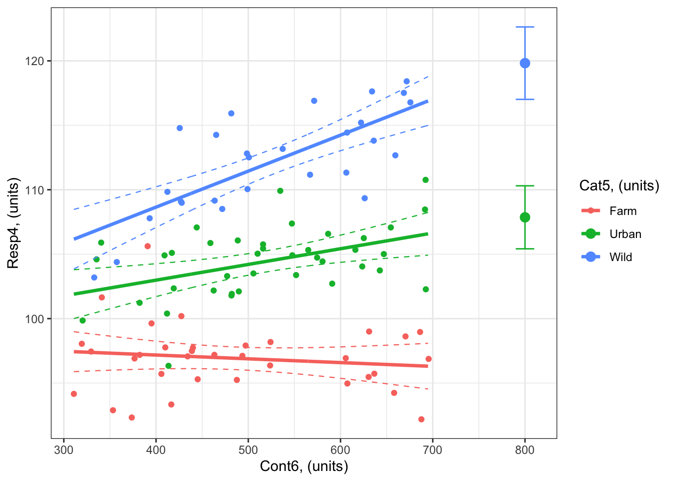

1.3 Inverse predicting for models with a binomial error distribution assumption

While the process (and code) above is identical regardless of your error distribution assumption, there is a second type of predicting one often uses when one has a model with a binomial error distribution assumption⁴.

Here, you are “inverse predicting” to predict the value of your predictor that will lead to a certain probability of your response being 1.

For example, you might want to know the amount of a toxin (your predictor) that leads to a 25% probability of dying⁵, or the age (your predictor) at which a fish has a 50% probability of being mature⁶.

One method to do this would be to predict your response at values of your predictor in high enough resolution so that you can pick out the appropriate predictor value. Here is an example where you want to know the value of Cont4 that will give a 75% probability of Resp3.b being 1, given your bestmod3.b of Resp3.b ~ Cont4 + 1:

forCont4<-seq(from = min(myDat3.b$Cont4), to = max(myDat3.b$Cont4), by = 0.01)# a sequence of numbers in your numeric predictor range, notice that you are using a very high resolution series of your predictor here.

forPred <- expand.grid(Cont4 = forCont4) # expand.grid() function makes sure you have all combinations of predictors.


## Step Two: Make your response prediction
myPred<-predict(bestMod3.b, # the model
                newdata = forPred, # the predictor values
                type = "link", # here, make the predictions on the link scale and we'll translate the back below
                se.fit = TRUE) # include uncertainty estimate

ilink <- family(bestMod3.b)$linkinv # get the conversion (inverse link) from the model to translate back to the response scale

### This can be added to our forPred data frame as:
forPred$Fit<-ilink(myPred$fit) # add your fit to the data frame
forPred$Lower<-ilink(myPred$fit - 1.96*myPred$se.fit) # add your uncertainty to the data frame, 95% confidence intervals
forPred$Upper<-ilink(myPred$fit + 1.96*myPred$se.fit) # add your uncertainty to the data frame, 95% confidence intervals

myPredDF <- data.frame(Cont4 = forCont4,
                       Fit = forPred$Fit,
                       Lower = forPred$Lower,
                       Upper = forPred$Upper)

myPredDF$Diff <- abs(myPred$fit - 0.75)

myInvPred <- myPredDF[which(myPredDF$Diff == min(myPredDF$Diff)),]

myInvPred

       Cont4       Fit     Lower     Upper        Diff
5094 81.9691 0.6790692 0.5899505 0.7568036 0.000502456

The estimate of Cont4 that leads to a 75% probability of Resp3.b being 1 is 0.7 units (95% confidence intervals: 0.59 to 0.76.

As you can see, this is a bit tedious. Another method would be to make a function yourself based on your statistical model equation and coefficients:

Note that your statistical model (GLM) with a binomial error distribution is:

\[ log_n(\frac{p}{1-p}) = \beta_0 + \beta_1 \cdot x \]

where $log_n(\frac{p}{1-p})$ is the logit function of the odds (see the Reporting section for more), $p$ is the probability at which you want a value of your predictor, $x$ is the value of your predictor, $\beta_0$ is your modelled intercept, and $\beta_1$ is your modelled slope (effect of your numeric predictor).

Inverse predicting means finding the value of $x$ that gives you a particular value of $p$. So we need to solve our equation for $x$:

\[\begin{align} log_n(\frac{p}{1-p}) &= \beta_0 + \beta_1 \cdot x\\[1em] log_n(\frac{p}{1-p}) - \beta_0 &= \beta_1 \cdot x\\[1em] \frac{log_n(\frac{p}{1-p}) - \beta_0}{\beta_1} &= x\\[1em] \end{align}\]

Then we can solve $x$ for a particular value of $p$. For example, what value of Cont4 will give a 75% probability of Resp3.b being 1, given your bestmod3.b of Resp3.b ~ Cont4 + 1:

# Make my inverse predicting function that is specific to this model:
funInvPred <- function (p, model) {
  modLink <- family(model)$linkfun # get the conversion (link) for the model
  (modLink(p) - coef(model)[["(Intercept)"]]) / coef(model)[["Cont4"]] # calculate x from p
}

# Apply the equation to estimate Cont4 when there is a 75% probability of Resp3.b being 1:
myInvPred <- funInvPred(p = 0.75, model = bestMod3.b) 

myInvPred

[1] 85.18394

The result is that you will have a 75% probability of Resp3.b being 1 if your Cont4 is r round(myInvPred,1) units. Note that there is no error estimated here. Generalized linear models assume that there is no error in your predictors, so getting the error on your inverse prediction is tricky and beyond the scope of this handbook.

Let’s finish here by adding our inverse prediction to the plot:

1.4 Up next

You did it! You made it through all the steps of our Statistical Modelling Framework. Nice work!

Up next we will practice applying the framework to new examples, and learn how to communicate the whole process in reports and papers.

Footnotes

In a previous section, we had the quote “All models are wrong but some are useful” to emphasize that models are approximation of the real world. Well, we can also say that “all data are wrong, but models can make data useful” (a quote by Andy Pershing) to emphasize that models are also needed to make generalizations and predictions about the systems that we are studying.↩︎
I realize that the term “prediction” and “predictor” can be confusing. Remember that another word for your model predictor is “covariate”.↩︎
note that when you hand a GLM object to predict(), R actually uses a function called predict.glm(). This does not affect what you need to do; it is just good to know in case you need help with the function↩︎
recall that this is also called “logistic regression”↩︎
sometimes called $LD_{25}$ where LD is lethal dose↩︎
sometimes called the $A_{50}$↩︎

1 Predicting

1.1 The process

Step Zero: consider your prediction limits

Step One: Define the predictor values for your response prediction

Step Two: Make your response prediction

1.2 Examples

Example 3: Resp3 ~ Cont4 + 1

What is the predicted response of Resp3 when Cont4 = 30?

What are the predicted responses of Resp3 when Cont4 = 9 and Cont4 = 22?

Example 4: Resp4 ~ Cat5 + Cont6 + Cat5:Cont6 + 1

Example: What is the predicted response of Resp4 when Cont6 = 800 for Cat5 = Urban?

Example: What is the predicted response of Resp4 when Cont6 = 800 for both Cat5 = Urban and Cat5 = Wild?

1.3 Inverse predicting for models with a binomial error distribution assumption

1.4 Up next

Footnotes

What is the predicted response of `Resp3` when `Cont4 = 30`?

What are the predicted responses of `Resp3` when `Cont4 = 9` and `Cont4 = 22`?

Example: What is the predicted response of `Resp4` when `Cont6 = 800` for `Cat5 = Urban`?

Example: What is the predicted response of `Resp4` when `Cont6 = 800` for both `Cat5 = Urban` and `Cat5 = Wild`?