You need to get your data into R in order to allow for data analysis.
How you can do it:
Importing your data from an external file
Most often, the data you will want to analyse are held in external files. You will need to import the data into R before you can work with it. Some things to consider:
Make your job easier with clean, understandable files
Data should be kept in long format with descriptive file names and an associated readme file. See your section on Data Collection and Curation for descriptions and tips on how to set you up for success.
Store your data in a known folder
To read in data, you first need to make sure your working directory (where R is currently “working”) is set to the right folder (i.e. the folder containing the data file(s) of interest). You can check your current working directory by typing getwd() at your command prompt and set your working directory with setwd(), e.g.
setwd("~/Desktop/StatsIntro")
As a starting point, keep your data file(s) in the same folder as your R script or markdown document.
Extra
You can also direct R to the folder with your data file(s) by including the path to the folder when you import the file.
Some users also like to use R Projects to keep all the files (data, scripts) in one place for a particular project. You can read more about R Projects here.
You can see what files are available in your current directory with listfiles(). For example, if you wanted a list of all .csv files in your working directory, you could type list.files(dir(), "*.csv") at the command prompt.
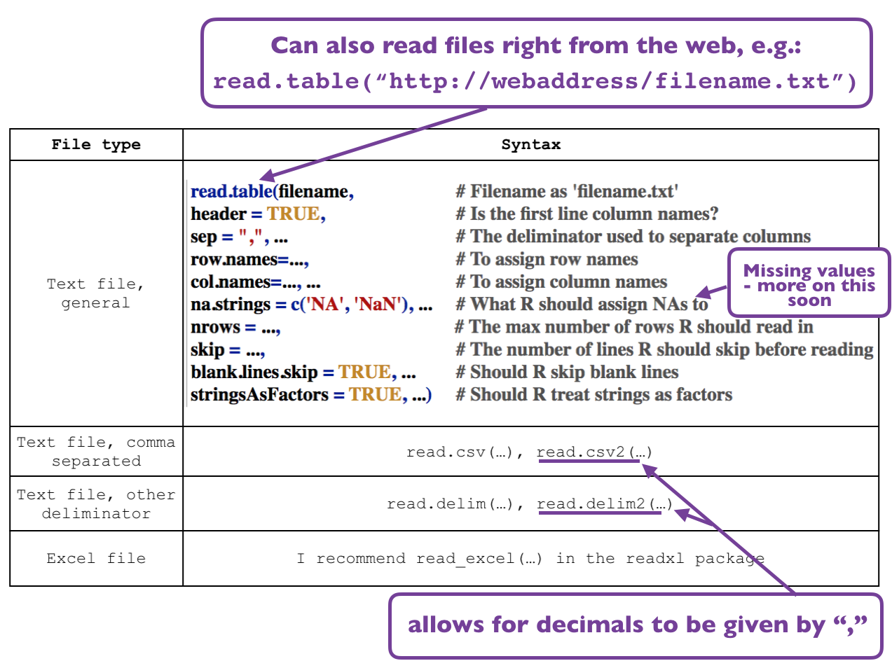
Read your data into R
R has a number of functions to help you get your data into R depending on the type and structure of your data file.
For example,
Here is an example of importing data from a .csv file:
# Reading in monthly chlorophyll data# Columns are:## Station: sampling station, either Halifax (HL2) or Saint John (S27)## Year: sampling year (4 digit)## Month: sampling month (numeric)## Temperature: average temperature (degC) in upper 50m.TData <-read.csv("ExampleData.csv", # name of data fileheader=TRUE) # make sure R sees column names (this is the default)head(TData) # take a look at the top few rows of the data
You have named the data object (TData). Without this, the data would be printed on the screen but not saved in your workspace. Note that you name (or assign) your object using an arrow <-.
The header=... argument is TRUE by default, and allows you to consider the first row in your data file as column names.
Quotations ("") are needed around the file name.
Note (as shown above) that you can break up a line of code on multiple lines so you can add comments after each argument.
aside: how computers store numbers
Computers store numbers as patterns of Os and 1s (“bits”). This system approximates decimals which can introduce rounding errors.
For example, \(\frac{1}{10}\) should be equal to 0.1:
1/10# is 0.1
[1] 0.1
but if you look at more decimal places, you can see 0.1 is not exactly 0.1 in R:
print(1/10, digits =20) # is not quite 0.1
[1] 0.10000000000000000555
The vast majority of time (99.99%) of the time, this will not cause a problem with your analysis. For the 0.01% of the time, it is important to understand that this precision error exists.
Manually entering data into R
When you import your data into R, it will most often be stored as a data table, which is a 2-dimensional (rows and columns) structure that can handle a variety of data types.
Learning about different data types and structures can help you understand how to work with data in R, and how to make these structures manually.
Caution
Importing your data file directly into R is much safer than manually typing in your data yourself. Humans cause errors.
Data types
Common data types or variables include:
numeric - this can include both numbers with decimals and integers (whole numbers)
character - text strings including letters or words. You must use quotes around character data to tell R it is a character.
factor - categorical variables that are stored as integers (representing the category number) and labels (representing the category name)
Extra
A fourth data type is “Logical”. This is how R stores true and false data.
Data structures
Here is a tour of data structures that are common to biological data analysis tasks. Note that you will primarily be using scalars, vectors and data frames.
Scalar:
Scalars are one dimensional and include only one value (or element). Here are a few examples:
Sc1 <-"banana"# a scalar containing a character valueprint(Sc1)
[1] "banana"
Sc2 <-45# a scalar containing a numeric integer valueprint(Sc2)
[1] 45
Sc3 <-3.2# a scalar containing a numeric decimal valueprint(Sc3)
[1] 3.2
Forcing the data type
R will normally guess the correct data type when you input or import data.
But sometimes R will get it wrong.
You can force R to see your data as a certain type (e.g. convert characters to factors) with:
factor() - to force data type factor
numeric() - to force data type numeric
character() - to force data type character
For example, the character scalar Sc1, can be converted to a factor with:
print(Sc1) # as character
[1] "banana"
Sc1 <-factor(Sc1) # convert to factorprint(Sc1) # now converted to factor
[1] banana
Levels: banana
Vector:
Vectors are a one-dimensional series of data values. Note that all elements (values) must be of the same data type (either numeric OR character OR factor).
The simplest way to make a vector is with the combine c() function. Here are a few examples:
V1 <-c("apple", "banana", "banana", "orange") # a vector containing character valuesprint(V1)
Another example: you might want to make a series of months repeating for four years. You can do this with the rep() function:
myMonths <-c("Jan", "Feb", "Mar") # define your monthsV5 <-rep(x = myMonths, # what you want repeatedtimes =4) # how many times you want it repeatedprint(V5)
# Note: this is the same as combining the two steps with ## V5 <- rep(x = c("Jan", "Feb", "Mar"), times = 4)# check ?rep for more options.
Matrix:
A matrix is a two-dimensional array (think rows and columns) that can only hold one type of data (either numeric OR character OR factor).
Array:
An array is a n-dimensional array that can only hold one type of data (either numeric OR character OR factor). For example, you can visualize a three-dimensional array as having rows, columns and different sheets.
Data frame:
A data frame is a two-dimensional array (think rows and columns) where each column can hold a different data type, so you can have numeric AND character AND factor data in the same sheet.
This is a very flexible data structure that you will use a lot in biology. In fact, when you import your data into R, it will most likely be automatically stored as a data frame.
Here is an example of manually creating a data frame. Note the comma , after each column definition:
DF1 <-data.frame(Year =rep(x =2021, times =3), # define your yearsMonth =c("Jan", "Feb", "Mar"), # define your monthsAbundance =c(43, 24, 5)) # abundance informationprint(DF1)
  Year Month Abundance
1 2021   Jan        43
2 2021   Feb        24
3 2021   Mar         5
Note that you can also add new columns to an existing data frame by giving the column a new name (one that is not already in the data frame):
DF1$Site <-"Mountain"print(DF1)
  Year Month Abundance     Site
1 2021   Jan        43 Mountain
2 2021   Feb        24 Mountain
3 2021   Mar         5 Mountain
List:
A list is a n-dimensional array that can only hold multiple types of data and elements that are different lengths.
Extra
There are many other types of data structures in R. Some other common ones are data tables (that are great for analysis on very large data sets, e.g. with many observations) and tibbles (that are data frames with a few extra features).
Naming your R objects
Naming (or “assigning”) your R objects should be done with the assignment symbol:
<-
as shown above.
The equals symbol = is used for defining arguments within a function (see more about this here).
Object names should be concise and meaningful - this will help with the readability of your code.
Official style guides urge users to use only combinations of lowercase letters, numbers when underscores (’_’) when naming objects. Note: you can not start your object name with a number
Use nouns (substantiver) to name data objects, and verbs (verber) to name functions1
Where possible, avoid using names of existing functions and variables. Doing so may cause confusion for the readers of your code.
For example, useful names:
wombat_data <- ...
day_1 <- ...
day_one <- ...
Avoid names like:
first_day_of_the_third_month <- ... (too long)
dayOne <- ... (Words are not separated by an underscore)2
9school <- ... (Can not start object name with a number)
dttjmc1 <- ... (Object name is not meaningful)
mean <- ... (reusing the name of an existing function)
Viewing your R objects
Note that you can print your object to the screen with the print() function or just by typing the object’s name.
To see all objects currently in your workspace, use ls().
You can also view data frames as a spreadsheet in R Studio using the View() function.
Removing your objects
You can remove a single object from your workspace with the rm() function. For example:
rm(V3)
will remove the V3 object from the workspace.
You can remove all objects in your workspace (clear your workspace) with rm(list = ls()).