Statistical Modelling: Communicating

In this chapter you will learn:
  • how to communicate motivations, methods and results of your data analysis and hypothesis testing for publication as a biological report/article

Communicating your hypothesis testing results

Here we will walk through your statistical modelling framework and discuss how to communicate motivations, methods and results of your data analysis and hypothesis testing for a biological report/article (& the exam!).

Here again is our statistical modelling framework:

A familiar example

I’ll use the following example case as I discuss how to communicate your results:

You are interested in moose (or elk, Alces alces) and how their growth rate changes from population to population. You find information on mean annual weight change by moose in 12 locations in Sweden. You wonder if latitude can explain some of the variability in growth rates you are observing. You also wonder if minimum winter temperature might explain some variability in growth rate. Finally, you wonder if changes in growth rate with latitude and/or winter temperature depend on each other (i.e, latitudinal dependent effects on growth rate depend on what the minimum winter temperature is) and/or sex (male and female) - i.e. the environmentally dependent change in growth rate depends on what sex the animal is.


And here’s a screenshot of the readme file for the moose data:

RESPONSE(S)

The task:

Your response variable is the observed variability you are trying to explain. Your response forms your research question - i.e. “why is my response varying?”. In this section, you need to identify the variability you are trying to explain and why (your motivation).

The code:

Code supporting your tasks in this section allow you to import your data and help you describe your response variable, e.g.:

rm(list=ls()) # make sure your workspace is clear

#Import the data
myDat <- read.table("ExDatComm.csv", # file name
                    sep = ',',  # lines in the file are separated by a comma - this information is in the README file
                    dec = '.', # decimals are denoted by '.' - this information is in the README file
                    stringsAsFactors = TRUE, # make sure strings (characters) are imported as factors
                    header = TRUE) # there is a column header in the file

str(myDat) # check the structure of the data file
'data.frame':   24 obs. of  6 variables:
 $ Study     : int  1 2 3 4 5 6 7 8 9 12 ...
 $ Sex       : Factor w/ 2 levels "Females","Males": 1 1 1 1 1 1 1 1 1 1 ...
 $ MassChange: num  10.2 8.7 11.2 9.4 6.2 10 14.1 12.2 16.2 13.6 ...
 $ DDLat     : num  58 57.7 58 57.9 59.8 61.6 62 62.7 64 65.5 ...
 $ WTemp     : num  -2.4 -1.7 -1.7 -1.7 -4.2 -5.6 -8.1 -7.7 -7.6 -9.3 ...
 $ Source    : Factor w/ 3 levels "Gothenburg","Lund",..: 2 3 3 2 3 2 1 1 3 3 ...
summary(myDat) # get summary information of each column
     Study            Sex       MassChange        DDLat           WTemp        
 Min.   : 1.00   Females:12   Min.   : 6.20   Min.   :57.70   Min.   :-11.900  
 1st Qu.: 3.75   Males  :12   1st Qu.:11.95   1st Qu.:58.00   1st Qu.: -8.400  
 Median : 6.50                Median :17.35   Median :61.80   Median : -6.600  
 Mean   : 7.00                Mean   :17.77   Mean   :61.60   Mean   : -6.100  
 3rd Qu.: 9.75                3rd Qu.:24.23   3rd Qu.:64.38   3rd Qu.: -2.225  
 Max.   :14.00                Max.   :30.60   Max.   :66.00   Max.   : -1.700  
        Source  
 Gothenburg: 6  
 Lund      : 8  
 Stockholm :10  


range(myDat$MassChange)
[1]  6.2 30.6

The write-up:

Use the code above, the data readme file, as well as supporting literature to communicate about your response variable and motivation. Include:

  • what your response variable is

  • why you want to explain variability in your response

  • your research question

  • how your response variable was measured and a description of how your response varies. For example, give the range in your response if possible. If your response is a category, give the levels of the category (e.g. alive vs. dead). Always give units, if applicable.

For example:

Here I want to explain variability in growth rate in moose (Alces alces). Moose size will be related to survival rates, and likely also their ability to reproduce (e.g. [@SandEtAl1995]). Being able to explain what controls growth rates in moose may help us explain why some populations are more productive than other populations, and it will help us predict productivity for populations at other places or times.

My research question is “why does growth rate vary?”. My observations of growth rate were measured from adult moose across 12 locations in Sweden. The growth rate varied from 6.2 to 30.6 kg per year.

PREDICTORS

The task:

Here you will identify the predictors in your model - i.e. what variables might explain variability in your response. To write-up this section, start with the biological mechanism (or process) that make you think the predictor could be influencing your response. Then describe how that predictor was measured. At this point you might identify mechanisms that you are not able to measure, e.g. because they were beyond the scope of your study. Make note of these. You will have a chance to talk about them as you discuss your results.

The code:

Code supporting your tasks in this section will help you describe your predictors, e.g.:

# Getting information on my predictors

range(myDat$DDLat) # ranges for continuous predictors
[1] 57.7 66.0
range(myDat$WTemp) # ranges for continuous predictors
[1] -11.9  -1.7
unique(myDat$Sex) # factor levels for categorical predictors
[1] Females Males  
Levels: Females Males

The write-up:

Use the code above, the data readme file, as well as supporting literature to communicate about your predictor variables. Include:

  • what your predictor variables are

  • why you think each predictor might explain variability in your response (mechanisms)

  • how each predictor variable was measured and a description of the predictor. This means at least giving the range of each predictor (for numeric predictors) or the levels of any categorical predictor. Remember to include units where applicable.

For example:

Here I consider the effects of latitude (˚N), minimum winter temperature (˚C) and sex (male vs. female) on annual growth in adult moose.

Latitude may impact the growth of the moose as the environment changes with latitude (e.g. temperature, food, light level, growing season). Differences in food availability may lead to growth differences [citation]1. In this study, latitude is measured in decimal degrees North and ranges from 57.7 to 66.0˚N.

Winter harshness may impact annual moose growth by making energetic losses larger in the winter due to increased costs of temperature regulation [citation]. Here, I measure winter harshness as minimum winter temperature (˚C) which ranged from -11.9 to -1.7˚C in my study.

Growth differences might also occur due to sex of the animal as male and female moose have different life history strategies (e.g. reproductive investment)[citation]. Here, I include effects of sex with observations of male vs. female for each growth rate measurement.

HYPOTHESIS

The task:

In this section you will describe your research hypothesis, first in human language, and then as an R model formula. Remember to communicate whether you will be including interactions along with main effects if you have more than one predictor.

The code:

No code needed here!

The write-up:

Use your answers to the previous sections to state your research hypothesis. Remember to consider interactions as well as the main effects. Include:

  • a description in words

  • a description in the formula notation

  • a definition of each term

For example,

I will test the research hypothesis that variability in adult moose growth rate (MassChange, kg per year) is explained by latitude (DDLat, ˚N), minimum winter temperature (WTemp, ˚C) and sex (Sex, male or female). I will test this by modelling:

MassChange ~ DDLat + WTemp + Sex + DDLat:Sex + WTemp:Sex + DDLat:WTemp + DDLat:WTemp:Sex

Note that “:” indicates an interaction among predictors. Here, I will test the main effects of each predictor on my response, as well as all possible interactions - i.e. whether latitudinal effects on moose growth vary between sexes (DDLat:Sex), minimum winter temperature effects on moose growth vary between sexes (WTemp:Sex), effects of minimum winter temperature on growth vary with latitude (DDLat:WTemp), and whether there is evidence that latitudinal effects of minimum winter temperature on growth differ between the sexes (DDLat:WTemp:Sex).

STARTING MODEL

The task:

This step involves describing how you built the statistical model to test your hypothesis. Here, you will:

  • Choose your error distribution assumption

  • Choose your shape assumption

  • Choose your starting model

  • Fit your starting model

The code:

Code supporting your tasks in this section will help you support your choices of your model assumptions, e.g.:

# Choosing your error distribution assumption:

## Understanding the nature of your response variable
summary(myDat$MassChange) # a summary description of MassChange
   Min. 1st Qu.  Median    Mean 3rd Qu.    Max. 
   6.20   11.95   17.35   17.77   24.23   30.60 
# Choosing your shape assumption:

## This can include plotting your response variable vs. each continuous predictor
### For DDLat:
library(ggplot2) # load ggplot2 library
ggplot()+ # start ggplot
  geom_point(data = myDat,
             mapping = aes(x = DDLat, y = MassChange))+ # add observations
  xlab("Latitude, ˚N")+ # change x-axis label
  ylab("Annual growth rate, kg per year")+ # change y-axis label
  labs(caption = "Figure 1: Observed annual growth rate (kg per year) vs. latitude (˚N)")+ # add figure caption
  theme_bw()+ # change theme of plot
  theme(plot.caption = element_text(hjust=0)) # move figure legend (caption) to left alignment. Use hjust = 0.5 to align in the center.

#### Relationship between DDLat and MassChange looks linear


### For WTemp:
ggplot()+ # start ggplot
  geom_point(data = myDat,
             mapping = aes(x = WTemp, y = MassChange))+ # add observations
  xlab("Minimum winter temperature, ˚C")+ # change x-axis label
  ylab("Annual growth rate, kg per year")+ # change y-axis label
  labs(caption = "Figure 2: Observed annual growth rate (kg per year) vs. minimum winter temperature (˚C)")+ # add figure caption
  theme_bw()+ # change theme of plot
  theme(plot.caption = element_text(hjust=0)) # move figure legend (caption) to left alignment. Use hjust = 0.5 to align in the center.

#### Relationship between WTemp and MassChange looks linear


# Fitting your starting model
startMod<-glm(formula = MassChange ~ DDLat + WTemp + Sex + DDLat:Sex + WTemp:Sex + DDLat:WTemp + DDLat:WTemp:Sex, # hypothesis
              data = myDat, # data
              family = gaussian(link = "identity")) # error distribution assumption

startMod

Call:  glm(formula = MassChange ~ DDLat + WTemp + Sex + DDLat:Sex + 
    WTemp:Sex + DDLat:WTemp + DDLat:WTemp:Sex, family = gaussian(link = "identity"), 
    data = myDat)

Coefficients:
         (Intercept)                 DDLat                 WTemp  
           -16.13632               0.43887               1.37886  
            SexMales        DDLat:SexMales        WTemp:SexMales  
           -54.84374               1.09654              -5.46475  
         DDLat:WTemp  DDLat:WTemp:SexMales  
            -0.02401               0.08799  

Degrees of Freedom: 23 Total (i.e. Null);  16 Residual
Null Deviance:      1200 
Residual Deviance: 75.09    AIC: 113.5

The write-up:

Use the code in the previous section as well as your theoretical understanding of the variables to communicate how you chose and fit your starting model. Include:

  • what your error distribution assumption is and how you chose it

  • what your shape assumption is and how you chose it

  • what type of model you chose for your starting model (e.g. GLM)

For example,

I built a model to test my hypothesis that variability in adult moose growth rate (MassChange, kg per year) is explained by latitude (DDLat, ˚N), minimum winter temperature (WTemp, ˚C) and sex (Sex, male or female). My error distribution assumption was normal (gaussian) as MassChange is continuous and can be positive or negative. My shape assumption regarding the relationship between MassChange and each predictor was linear. This was chosen after inspecting plots of MassChange and both WTemp and DDLat (Figures 1 & 2). Plots were made using the ggplot2 package (@Wickham2016)2 In addition, a linear shape assumption was chosen to describe the relationship between Sex and MassChange as Sex is a categorical variable.

Based on these assumption I tested my hypothesis by fitting a generalized linear model to my data with normal error distribution assumption and identity link3. All model fitting and analysis was done in R (@RCite).4

MODEL VALIDATION

The task:

Here, you will describe how you assessed your model to ensure that it can be used to test your hypothesis. Remember that the assumptions you made above (error distribution & shape assumptions) were a “best guess” but it is only after the model is fit that we can confirm that it is useful. In this section you will:

  • Consider predictor collinearity

  • Consider observation independence

  • Consider your error distribution assumption

  • Consider your shape assumption

and report your results.

The code:

Code supporting your tasks in this section will help you assess your model for violations that may make it invalid for testing your hypothesis, e.g.:

# Consider predictor collinearity 
## Fit a model without interactions
startMod.noInt <- glm(formula = MassChange ~ DDLat + WTemp + Sex, # hypothesis
              data = myDat, # data
              family = gaussian(link = "identity")) # error distribution assumption

startMod.noInt

Call:  glm(formula = MassChange ~ DDLat + WTemp + Sex, family = gaussian(link = "identity"), 
    data = myDat)

Coefficients:
(Intercept)        DDLat        WTemp     SexMales  
    -43.013        0.879       -0.105       12.000  

Degrees of Freedom: 23 Total (i.e. Null);  20 Residual
Null Deviance:      1200 
Residual Deviance: 99.43    AIC: 112.2
## Calculate Variance Inflation Factors (VIFs)
library(car) # load the car package
Loading required package: carData
vif(startMod.noInt) # estimate VIFs
   DDLat    WTemp      Sex 
23.08925 23.08925  1.00000 
## there are VIF values higher than the threshold value (in this case VIFs > 3).  Let's remove WTemp and recalculate the VIFs:

startMod.noInt.noWTemp <- glm(formula = MassChange ~ DDLat + Sex, # hypothesis
              data = myDat, # data
              family = gaussian(link = "identity")) # error distribution assumption

startMod.noInt.noWTemp

Call:  glm(formula = MassChange ~ DDLat + Sex, family = gaussian(link = "identity"), 
    data = myDat)

Coefficients:
(Intercept)        DDLat     SexMales  
   -49.5975       0.9963      12.0000  

Degrees of Freedom: 23 Total (i.e. Null);  21 Residual
Null Deviance:      1200 
Residual Deviance: 99.58    AIC: 110.3
## Recalculating the VIFs

# vif(startMod.noInt.noWTemp) # estimate VIFs

## there are no longer any problems with predictor collinearity, as all VIFs < 3

## Refitting your starting model with the interactions back in:
startMod <- glm(formula = MassChange ~ DDLat + Sex + DDLat:Sex, # hypothesis
              data = myDat, # data
              family = gaussian(link = "identity")) # error distribution assumption


# Consider observation independence
## You wonder if Source could be violating your observation independence assumption.  Check to see with a plot of your residuals vs. Source

library(DHARMa) # load package
This is DHARMa 0.4.7. For overview type '?DHARMa'. For recent changes, type news(package = 'DHARMa')
simOut <- simulateResiduals(fittedModel = startMod, n = 250) # simulate data from our model n times and calculate residuals

myDat$myResid <- simOut$scaledResiduals # add residuals to data frame

## plot study vs. residuals

ggplot()+ # initialize plot
  geom_violin(data = myDat, 
              mapping = aes(x = Source, y = myResid)) + # add a violin plot
  xlab("data source university (no units)")+ # change x-axis label
  ylab("scaled residuals (no units)")+ # change y-axis label
  labs(caption = "Figure 3: Comparing model residuals across data sources") + # add figure caption
  theme_bw()+ # change theme of plot
  theme(plot.caption = element_text(hjust=0)) # move figure legend (caption) to left alignment. Use hjust = 0.5 to align in the center.

testCategorical(simulationOutput = simOut, # compare simulated residuals
     catPred = myDat$Source)

$uniformity
$uniformity$details
catPred: Gothenburg

    Exact one-sample Kolmogorov-Smirnov test

data:  dd[x, ]
D = 0.22667, p-value = 0.8568
alternative hypothesis: two-sided

------------------------------------------------------------ 
catPred: Lund

    Exact one-sample Kolmogorov-Smirnov test

data:  dd[x, ]
D = 0.188, p-value = 0.8937
alternative hypothesis: two-sided

------------------------------------------------------------ 
catPred: Stockholm

    Exact one-sample Kolmogorov-Smirnov test

data:  dd[x, ]
D = 0.268, p-value = 0.398
alternative hypothesis: two-sided


$uniformity$p.value
[1] 0.8567934 0.8936603 0.3980193

$uniformity$p.value.cor
[1] 1 1 1


$homogeneity
Levene's Test for Homogeneity of Variance (center = median)
      Df F value Pr(>F)
group  2  0.5726 0.5726
      21               
# Consider your error distribution assumption
plotQQunif(simulationOutput = simOut, # the object made when estimating the scaled residuals.  See section 2.1 above
           testUniformity = TRUE, # testing the distribution of the residuals 
           testOutliers = TRUE, # testing the presence of outliers
           testDispersion = TRUE) # testing the dispersion of the distribution

# Consider your shape assumptions

# A plot of residuals vs. fitted values
plotResiduals(simulationOutput = simOut, # the object made when estimating the scaled residuals.  See section 2.1 above
              form = NULL) # the variable against which to plot the residuals.  When form = NULL, we see the residuals vs. fitted values

plotResiduals(simulationOutput = simOut, # compare simulated data to 
     form = myDat$DDLat, # our observations
     asFactor = FALSE) # whether the variable plotted is a factor

plotResiduals(simulationOutput = simOut, # compare simulated data to 
     form = myDat$Sex, # our observations
     asFactor = TRUE) # whether the variable plotted is a factor

# define my validated model

validMod <- startMod

The write-up:

Use the code in the previous section to comment on your model’s validity in testing your research hypothesis. Include:

  • how you determined if there were problems with predictor collinearity and any actions you took if you detected a problem

  • how you determined if there were problems with observation dependence and any actions you took if you detected a problem

  • how you determined if your error distribution assumption was valid and any actions you took to address problems

  • how you determined if your shape assumption was valid and any actions you took to address problems

For example,

I tested if collinearity among my predictors was making my model coefficients uncertain by estimating variance inflation factors (VIFs) with the car package (@FoxWeisberg2019_car)5. Initial VIFs for DDLat and WTemp were > 23 indicating a high level of predictor collinearity. WTemp was removed from the model and the VIFs were re-estimated. VIFs in the new model were both 1, and it was concluded that there was no further issue with predictor collinearity.

The new starting model will test the hypothesis:

MassChange ~ Latitude + Sex + Latitude:Sex

I tested my assumption of observation independence by determining if the observations were grouped by Source (the source university for the data6). I estimated my model residuals using the DHARMA package (@Hartig2022_DHARMa)7 and plotted my residuals vs. Source. I tested for patterns in the residuals due to Source by the Levene test for the homogeneity of variances. There was no evidence that the observations were dependent on Source (Levene test, P = 0.573) concluded my data were not dependent on one another based on Source as the residuals were evenly distributed across the three source universities (see Figure 3).

I assessed my error distribution assumption by inspected my residuals. Observed residuals were similar to those expected given my normal error distribution assumption. The Kolmogorov-Smirnov test comparing the observed to the expected distribution was not significant (P = 0.96). The dispersion and outlier tests were also not significant (P = 0.74 and P = 0.99 respectively). From these results, I concluded that my error distribution assumption was appropriate.

I assessed my shape assumption by inspected my residuals vs. each predictor. My residuals were evenly distributed with Latitude, indicating a linear shape assumption for Latitude was appropriate. The linear shape assumption for Sex was necessary as Sex is a categorical variable. A plot of the residuals vs. Sex showed residuals were evenly distributed across the two sexes. From these results, I concluded that my linear shape assumptions were appropriate.

Given these results, I determined that the new starting model (MassChange ~ Latitude + Sex + Latitude:Sex) can be used to test my hypothesis.

HYPOTHESIS TESTING

The task:

Here, you will use your model to test your hypothesis. For the purposes of this course, you will do this with the model selection method we practiced in class8. In this section you will:

  • fit and compare models representing all possible combinations of the predictors in your starting model

  • use the results to choose best-specified model(s)

  • report your results.

The code:

Code supporting your tasks in this section will help you test and rank your models, e.g.:

library(MuMIn) # load package

options(na.action = "na.fail") # needed for dredge() function to prevent illegal model comparisons

(dredgeOut<-dredge(validMod, extra = "R^2")) # fit and compare a model set representing all possible predictor combinations
Fixed term is "(Intercept)"
Global model call: glm(formula = MassChange ~ DDLat + Sex + DDLat:Sex, family = gaussian(link = "identity"), 
    data = myDat)
---
Model selection table 
   (Int)    DDL Sex DDL:Sex    R^2 df  logLik  AICc delta weight
8 -31.60 0.7041   +       + 0.9340  5 -48.387 110.1  0.00  0.756
4 -49.60 0.9963   +         0.9170  4 -51.130 112.4  2.26  0.244
3  11.78          +         0.7200  3 -65.726 138.7 28.54  0.000
2 -43.60 0.9963             0.1971  3 -78.366 163.9 53.82  0.000
1  17.78                    0.0000  2 -80.999 166.6 56.46  0.000
Models ranked by AICc(x) 
# You can make a pretty table to use in your write-up
library(gt) # load gt package

myTable <- gt(dredgeOut) # make a pretty table
myTable <- fmt_number(myTable, # to format the numbers in my table
                    columns = everything(), # which columns to format
                    decimals = 2) # round to 2 decimal places
myTable <- tab_caption(myTable, 
                       caption = "Table 1: Model selection table for hypothesis testing. Each row is a model fit to my data. predictors included in each model are indicated by a number (for continuous predictors and intercept) or '+' (for categorical predictors). R^2 is the likelihood ratio R-squared, df indicates number of model parameters, logLik is the model Log-likelihood, AICc is the corrected Akaike Information Criteria, delta is the change in AICc between the model and that of the lowest AICc, and weight is the Akaike weights.")

myTable
Table 1: Model selection table for hypothesis testing. Each row is a model fit to my data. predictors included in each model are indicated by a number (for continuous predictors and intercept) or '+' (for categorical predictors). R^2 is the likelihood ratio R-squared, df indicates number of model parameters, logLik is the model Log-likelihood, AICc is the corrected Akaike Information Criteria, delta is the change in AICc between the model and that of the lowest AICc, and weight is the Akaike weights.
(Intercept) DDLat Sex DDLat:Sex R^2 df logLik AICc delta weight
−31.60 0.70 + + 0.93 5.00 −48.39 110.11 0.00 0.76
−49.60 1.00 + NA 0.92 4.00 −51.13 112.36 2.26 0.24
11.78 NA + NA 0.72 3.00 −65.73 138.65 28.54 0.00
−43.60 1.00 NA NA 0.20 3.00 −78.37 163.93 53.82 0.00
17.78 NA NA NA 0.00 2.00 −81.00 166.57 56.46 0.00
## Could also be written as:
 # dredgeOut %>%
 #   gt() %>% # make a pretty table
 #   fmt_number(columns = everything(), # which columns to format
 #                     decimals = 2) %>% # round to 2 decimal places
 #   tab_caption(caption = "Table 1: Model selection table for hypothesis testing. Each row is a model fit to my data. predictors included in each model are indicated by a number (for continuous predictors and intercept) or '+' (for categorical predictors). R^2 is the likelihood ratio R-squared, df indicates number of model parameters, logLik is the model Log-likelihood, AICc is the corrected Akaike Information Criteria, delta is the change in AICc between the model and that of the lowest AICc, and weight is the Akaike weights.")

The write-up:

Use the code in the previous section to explain how you chose your best-specified model. Include:

  • the method you are using to test your hypothesis

  • how you fit and rank your candidate model set

  • how you made your decision regarding your best-specified model

For example,

I used model selection to test my hypothesis that variability in adult moose growth rate is explained by latitude, sex and the interaction between the latitude and sex. I used the dredge() function from the MuMIn package (@Barton2022_MuMIn) to fit and rank models representing all possible predictor combinations. Models were ranked by corrected Akaike Information Criteria9 which [add a brief description of what AICc is - see here for more].10

The model with the lowest AICc was chosen as the best-specified model, with models within ∆AICc = 2 of the lowest AICc model being considered equally best-specified.

The best-specified model was the full model:

MassChange ~ DDLat + Sex + DDLat:Sex

with an Akaike weight (normalized relative likelihood) of 0.756. The next best model had an AIC of 2.26 more than the top model and an Akaike weight of 0.244.

REPORTING

The task:

In this section, you will report your hypothesis testing results. Specifically,

  • Report your best-specified model(s): Report your best-specified model and communicate the terms (predictors and interactions) that are in your model, and the terms that were in your starting model that are not in your best-specified model.

  • Report how well your model explains your response: Report how much deviance in your reponse your model explains. If you have more than one predictor, you should also report how important each term is in explaining the deviance.

  • Report your modelled effects: Report your effects visually and quantitatively.

The code:

Code supporting your tasks in this section will help you communicate what your results tell you about your hypothesis, e.g.:

Reporting your best-specified model(s)

# Report your best-specified model(s)


## Our best-specified model is MassChange ~ DDLat + Sex + DDLat:Sex (model #8 in the dredge() output).

bestMod<-(eval(attr(dredgeOut, "model.calls")$`8`)) # extract model #8 from dredge table

Reporting how well your model explains your response

## Report explained deviance

r.squaredLR(bestMod) # estimates the likelihood ratio R^2.  Could also estimate a traditional R^2 with 1-summary(bestMod)$deviance/summary(bestMod)$null.deviance here as the error distribution assumption is normal and the shape assumption is linear, but the likelihood ratio R^2 function is generally applicable to many error distribution assumptions and equivalent to the traditional R^2 when the error distribution assumption is normal and the shape assumption is linear.
[1] 0.9339728
attr(,"adj.r.squared")
[1] 0.9350677
## Report how important each model term (predictor fixed effects and any interactions) is in explaining the deviation in your response. 
sw(dredgeOut)
                     Sex  DDLat DDLat:Sex
Sum of weights:      1.00 1.00  0.76     
N containing models:    3    3     1     

Visualizing your model effects

# Set up your predictors for the visualized fit
forLat<-seq(from = min(myDat$DDLat), 
             to = max(myDat$DDLat), 
             by = 1) # get a range of latitudes for making predictions
forSex<-unique(myDat$Sex) # get every level of my Sex predictor
forVis<-expand.grid(DDLat=forLat, Sex=forSex) # create a data frame with all combinations of predictors

# Get your model fit estimates at each value of your predictors
modFit<-predict(bestMod, # the model
                newdata = forVis, # the predictor values
                type = "link",# here, make the predictions on the link scale and we'll translate the back below
                se.fit = TRUE) # include uncertainty estimate

ilink <- family(bestMod)$linkinv # get the conversion (inverse link) from the model to translate back to the response scale

forVis$Fit<-ilink(modFit$fit) # add your fit to the data frame
forVis$Upper<-ilink(modFit$fit + 1.96*modFit$se.fit) # add your uncertainty to the data frame, 95% confidence intervals
forVis$Lower<-ilink(modFit$fit - 1.96*modFit$se.fit) # add your uncertainty to the data frame


myPlot <- ggplot()+
  geom_point(data = myDat, # data
             mapping = aes(x = DDLat, y = MassChange, col = Sex))+ # add data to your plot
  geom_ribbon(data = forVis, 
              mapping = aes(x = DDLat, ymin = Lower, ymax = Upper, fill = Sex), alpha = 0.5)+ # add the uncertainty to your plot
  geom_line(data = forVis, 
            mapping = aes(x = DDLat, y = Fit, col = Sex))+ # add the model fit to your plot
  ylab("Change in body mass (kg per year)")+ # change y-axis label
  xlab("Latitude (˚N)")+ # change x-axis label
  labs(caption = "Figure 4: Modelled effects (lines, mean with 95% confidence interval) of latitude and sex (colours) on growth rate \nalong with observations (points)")+
  theme_bw()+ # change ggplot theme
  theme(plot.caption = element_text(hjust=0)) # move figure legend (caption) to left alignment. Use hjust = 0.5 to align in the center.

myPlot

# to save the ggplot 
ggsave(filename = "myPlot.png", # filename
       plot = myPlot) # plot to save
Saving 7 x 5 in image

Quantifying your model effects

For each categorical predictor:

  • the modelled response on the RESPONSE scale for each level in your categorical predictor

  • the evidence that the modelled response is different across levels of your categorical predictor

### Find the effects for Sex.  As Sex is categorical, we do this for emmeans() and the reported coefficients are predicted mean response at each level of Sex. 

library(emmeans) # load emmeans package
Welcome to emmeans.
Caution: You lose important information if you filter this package's results.
See '? untidy'
#### the modelled response on the linked scale for each level in your categorical predictor
emmOutLink <- emmeans(object = bestMod, # your model
                      specs = ~ DDLat + Sex + DDLat:Sex + 1, # your predictors
                      type = "link") # report coefficients on the response scale

emmOutLink
 DDLat Sex     emmean    SE df lower.CL upper.CL
  61.6 Females   11.8 0.575 20     10.6       13
  61.6 Males     23.8 0.575 20     22.6       25

Confidence level used: 0.95 
#### the modelled response on the response scale for each level in your categorical predictor
emmOut <- emmeans(object = bestMod, # your model
                  specs = ~ DDLat + Sex + DDLat:Sex + 1, # your predictors
                  type = "response") # report coefficients on the response scale

emmOut # note that the link and response scale here are identical because we are using an identity link.
 DDLat Sex     emmean    SE df lower.CL upper.CL
  61.6 Females   11.8 0.575 20     10.6       13
  61.6 Males     23.8 0.575 20     22.6       25

Confidence level used: 0.95 
#### the evidence that the modelled response is different across levels of your categorical predictor.  Are the effects of Sex different from each other?
pairs(emmOut, # emmeans object
      simple = "Sex") # simple comparison by Sex
DDLat = 61.6:
 contrast        estimate    SE df t.ratio p.value
 Females - Males      -12 0.813 20 -14.768  <.0001
  • for each numeric predictor:

  • the effect on your response of a unit change in your numeric predictor on the RESPONSE scale

  • if there is an interaction: report how the interaction shows up in your modelled effects, making comparison across levels of a categorical predictor as appropriate (see example)

## the effect on your response of a unit change in your continuous predictor on the LINK scale

### Find the coefficients for Latitude.  As Latitude is continuous, we do this with emtrends() and the reported coefficients are the slope describing the change in predicted mean response with a unit change in Latitude.  Note that emtrends() reports coefficients on the LINK scale.  You need to convert this to the response scale.  In our case, the error distribution assumption is normal so nothing needs to be done to convert the coefficients.
trendsOut <- emtrends(object = bestMod, # your model
                      specs = ~ DDLat + Sex + DDLat:Sex, # your predictors
                      var = "DDLat") # name of your continuous predictor

trendsOut
 DDLat Sex     DDLat.trend    SE df lower.CL upper.CL
  61.6 Females       0.704 0.182 20    0.324     1.08
  61.6 Males         1.289 0.182 20    0.908     1.67

Confidence level used: 0.95 
## the effect on your response of a unit change in your continuous predictor on the RESPONSE scale
### Note that emtrends() reports coefficients on the LINK scale.  You need to convert this to the response scale.  In our case, the error distribution assumption is normal so nothing needs to be done to convert the coefficients.

## report how the interaction shows up in your modelled effects, making comparison across levels of a categorical predictor as appropriate (see example)
#### Are the effects of DDLat different from each other across Sex?
pairs(trendsOut, # trendsOut object
      simple = "Sex") # simple comparisons by Sex
DDLat = 61.6:
 contrast        estimate    SE df t.ratio p.value
 Females - Males   -0.584 0.258 20  -2.266  0.0347

The write-up:

Use the results of the code above to report your hypothesis testing results. Include:

  • a description of the terms (predictor fixed effects and any interactions) that are in your best-specified model

  • a comparison these terms to your starting model - are all terms in your starting model in you best-specified model?

  • how much deviance in your response is explained by your model

  • how important each term (predictor or interaction) is in explaining the deviance in your response

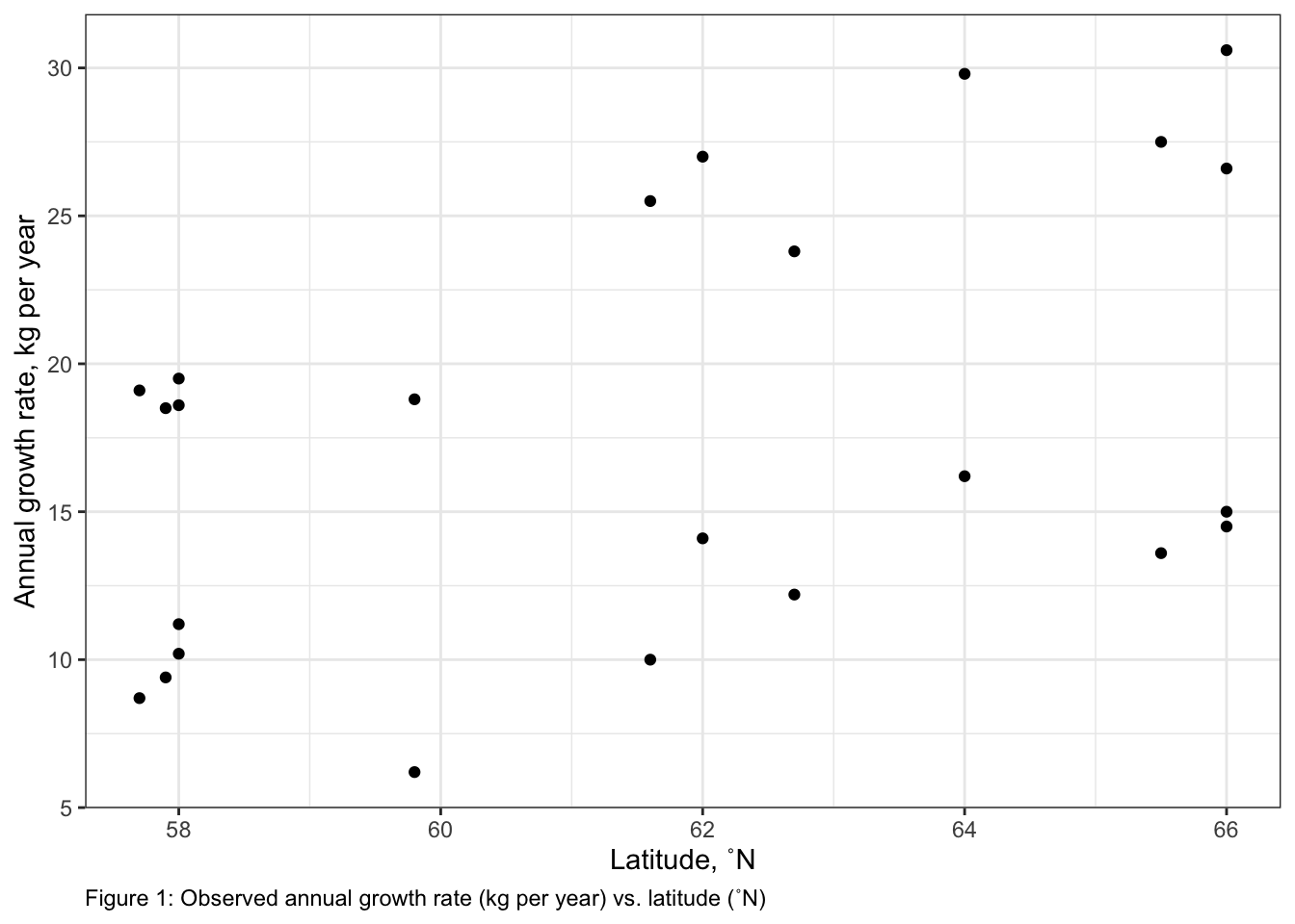
  • a visual representation of your modelled effects (a plot): Remember to include your model predictions, uncertainty as well as your observations. Include units on your axes and a figure number and legend.

  • a report of your modelled effects quantitatively by reporting coefficients on the response scale:

    • for each categorical predictor:

      • the modelled response on the RESPONSE scale for each level in your categorical predictor

      • the evidence that the modelled response is different across levels of your categorical predictor

    • for each continuous predictor:

      • the effect on your response of a unit change in your numeric predictor on the RESPONSE scale

      • if there is an interaction: report how the interaction shows up in your modelled effects, making comparison across levels of a categorical predictor as appropriate (see example)

  • linking the modelled effects back to the mechanisms

  • consider what might be explaining the remaining (unexplained) deviation in your response

For example,

My best-specified model tells me that the growth varies with latitude and sex, and that the effect of latitude on growth varies with sex11. The terms in my best-specified model are the same as those in my starting model indicating that there is evidence that the main effects of latitude and sex as well as the interaction are explaining variability in moose growth.

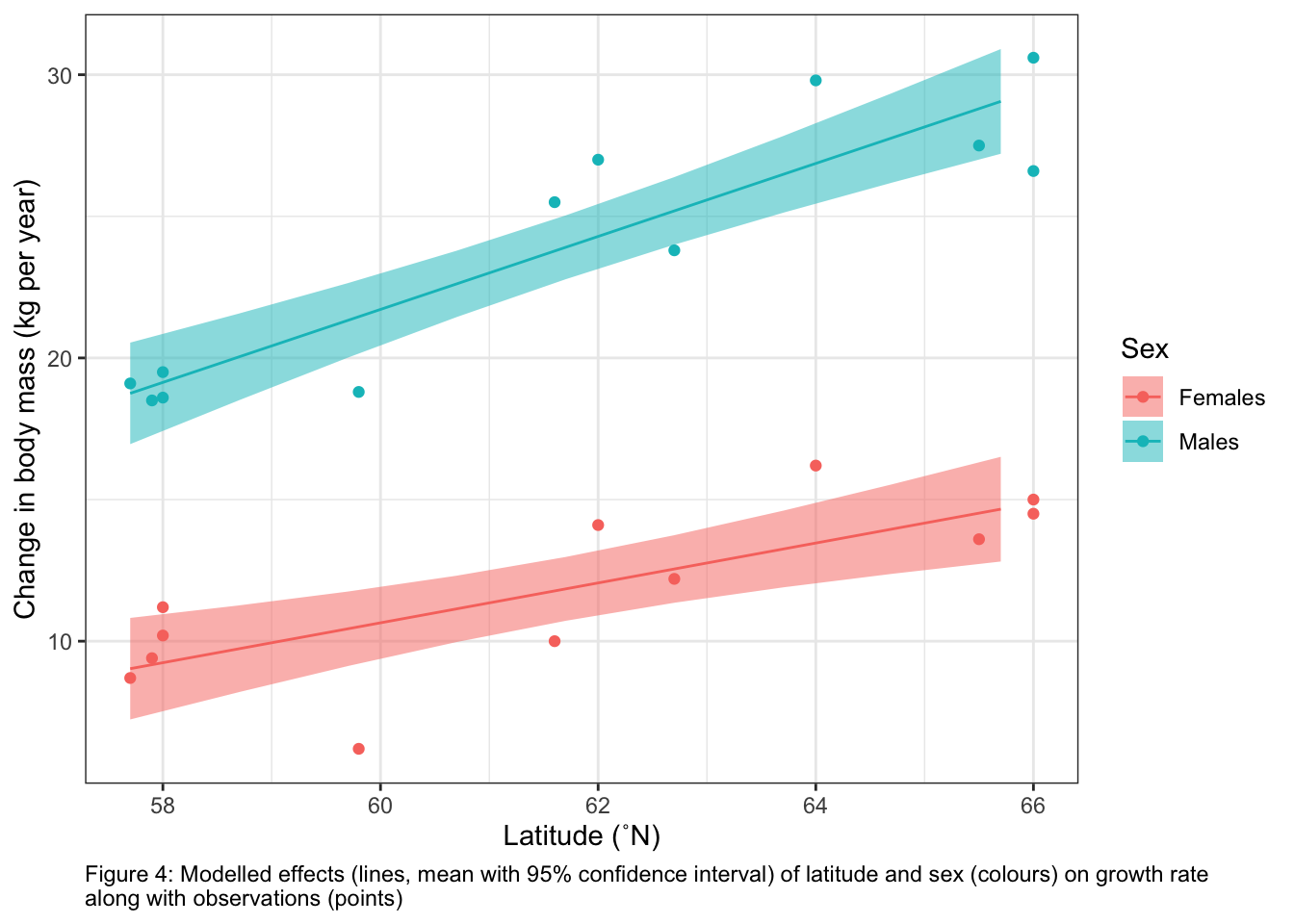
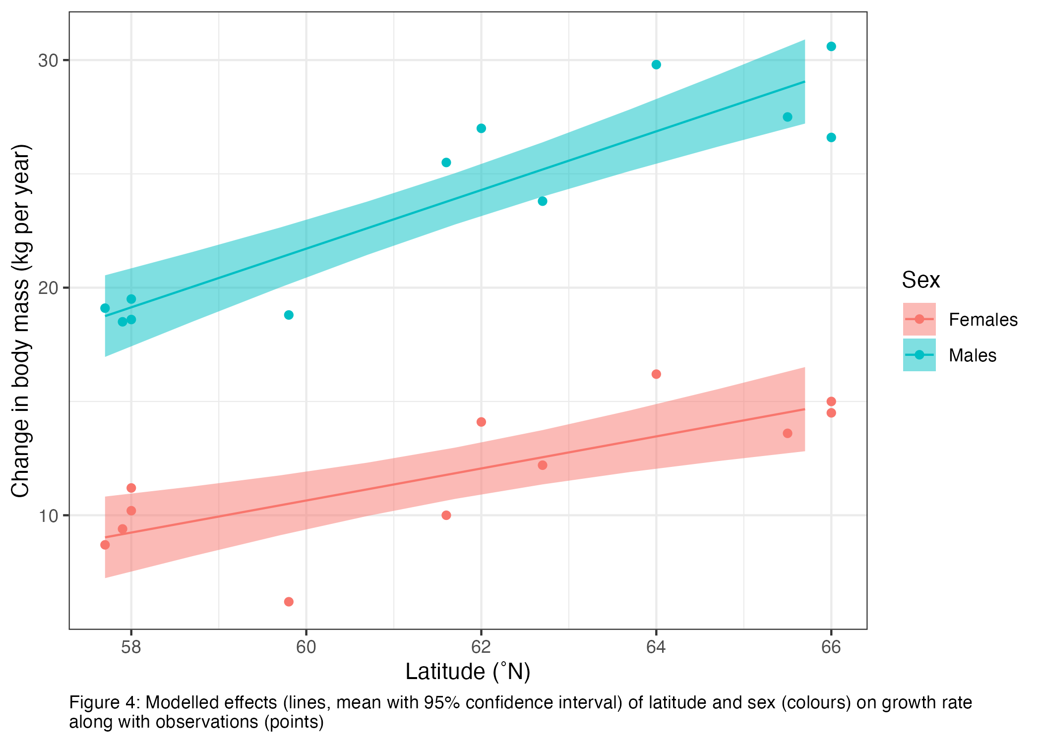
Growth rate is higher for males than females: the predicted growth when latitude is 61.6˚N (the mean of the latitudinal range) is 11.8 ± 0.6 kg year-1 for females and 23.8 ± 0.6 kg year-1 for males.12. There is evidence the predictions of growth between sexes are different (t-test; t-ratio = -14.8; P < 0.0001). Note that these estimates are the same on the link and response scales as the model uses an identity link.

The coefficient (slope) for the effect of a change of latitude on the growth rate is 0.70 ± 0.18 kg year-1 ˚N-1 for females and 1.29 ± 0.18 kg year-1 ˚N-1 for males. There is evidence that these effects (slopes) are different from one another (t-test, t-ratio = -2.3, P = 0.035). These coefficients show that growth rates increase with latitude for both sexes, but that the effect of latitude on growth is higher for male vs. female moose. Note that these estimates are the same on the link and response scales as the model uses an identity link.

Figure 4 shows the modelled effects of latitude and sex on growth rate along with my observations.

Together the effects of latitude and sex explain 93% of the deviance in growth rate (Likelihood ratio R2).13.

Based on the sum of Akaike weights, latitude and sex are equally important in explaining the deviance in growth rate as they appear in all models with Akaike weights > 0. The interaction between latitude and sex is slightly less important appearing only in the best-specified model with an Akaike weight of 0.76.

An increase in annual growth rate with latitude may indicate… [link to mechanisms].

A sex-specific increase in annual growth rate may indicate… [link to mechanisms].

[a discussion on study limitations (e.g. how the growth rate, latitude, etc. were measured)].

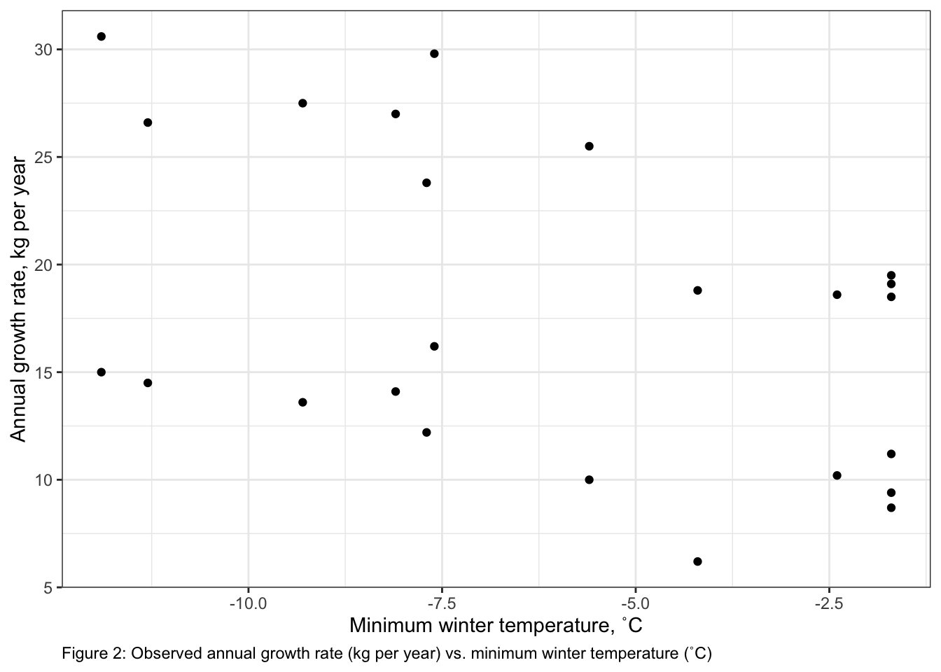
The remaining unexplained deviance may be due to other factors affecting growth rate such as winter harshness, food availability, etc. Note that I was not able to include minimum winter temperature in my hypothesis test due to high collinearity between latitude and minimum winter temperature. Therefore, I do not know if the measured latitudinal effect on growth might mechanistically be due to winter harshness (here estimated as minimum winter temperature). This could be tested if I was able to expand my data set to include sites where latitude and minimum winter temperature were less correlated… [discussion on other, untested factors that may be responsible for the unexplained deviance].

PREDICTING

The task:

Here you may use your model to make predictions (remembering prediction limits). For the assignments and exam, we will explicitly ask you to make a prediction if we want to see one.

If you want to make a prediction (e.g. “based on your best-specified model, what is your predicted mean annual growth of a female moose living in Sicily, Italy?”), in this section you want to report your prediction results and give any limitations to the prediction.

The code:

Code supporting your tasks in this section will help you communicate what prediction you made and the results, e.g.:

# Based on your best-specified model, what is your predicted mean annual growth of an adult female moose living in Sicily, Italy?

## Looking on the internet, we see that Sicily, IT is at 37.6˚N.

## Step One: Define the predictor values for your response prediction
forPred <- data.frame(Sex = "Females", DDLat = 37.6) # values of the predictors at which to make the prediction

## Step Two: Make your response prediction
predResp <- predict(bestMod, # the model
                newdata = forPred, # the predictor values
                type = "link",# here, make the predictions on the link scale and we'll translate the back below
                se.fit = TRUE) # include uncertainty estimate

ilink <- family(bestMod)$linkinv # get the conversion (inverse link) from the model to translate back to the response scale

forPred$Resp<-ilink(predResp$fit) # add your fit to the data frame
forPred$Upper<-ilink(predResp$fit + 1.96*predResp$se.fit) # add your uncertainty to the data frame, 95% confidence intervals
forPred$Lower<-ilink(predResp$fit - 1.96*predResp$se.fit) # add your uncertainty to the data frame

forPred
      Sex DDLat      Resp    Upper     Lower
1 Females  37.6 -5.122918 3.529435 -13.77527

The write-up:

Use the code in the previous section to present the results of your prediction. Include

  • the prediction and an estimate of uncertainty

  • any perceived prediction limits.

For example,

I used my best-specified model to estimate the mean annual growth rate of adult female moose living in Sicily, Italy (~ 37.6˚N) as -5.1 kg per year (95% confidence interval: -14 to 3.5 kg per year). While this is an estimate consistent with my model, it likely is unrealistic as the distribution of moose does not currently extend as far south as Sicily. It is likely there are limitations to their dispersal to or survival in this area and my model may not be valid for latitudes so far south (as evidenced by the predicted negative growth).

Commenting your code

Finally, let’s talk about commenting your code.

Why comment

Commenting your code (using #) allows you to clarify what your R code is doing at each step. This will help you when you share your code with collaborators and it will help you catch errors in your code. Commenting will also help you make your code useful to yourself for future projects. Remember that your closest collaborator is yourself six months ago and they don’t return emails!

How to comment

Clarify each line of your code by adding a # and then a description of what the code is doing. Don’t just write the function name in your comments. Add (in human language) what that line of code is doing. Use your comments to:

  • Define variables, e.g.
forSex<-unique(myDat$Sex) # get every level of my Sex predictor
  • Explain what the code is trying to do, e.g.
# Get your model fit estimates at each value of your predictors
modFit<-predict(bestMod, # the model
                newdata = forVis, # the predictor values
                type = "response", # make the predictions on the response scale
                se.fit = TRUE) # include uncertainty estimate
  • Explain why you chose a particular strategy, e.g.
r.squaredLR(bestMod) # estimates the likelihood ratio R^2.  Could also estimate a traditional R^2 with 1-summary(bestMod)$deviance/summary(bestMod)$null.deviance here as the error distribution assumption is normal and the shape assumption is linear, but the likelihood ratio R^2 function is generally applicable to many error distribution assumptions and equivalent to the traditional R^2 when the error distribution assumption is normal and the shape assumption is linear.

From Hypothesis Testing to Scientific Paper

In this final section, we talk about how to take all the pieces from your statistical modelling adventure to create a scientific report and paper.

Introduction

Methods

Results

Discussion

Up Next

In the next chapter, we will discuss how the GLM methods we have been using relate to other types of statistical models. This will help you communicate your choices and methods to others that may differ in the way they are approaching their statistical modelling.

Copyright 2025, DSP Taskforce

Footnotes

  1. here, I’ll write “citation” where you would support your statements with the existing literature↩︎

  2. find this citation with citation("ggplot2")↩︎

  3. note that a GLM with a normal error distribution assumption is also called a linear model. This is covered in “How GLMs relate to other types of models”↩︎

  4. you can find which version of R you are using with citation() (nothing inside the parentheses)↩︎

  5. you can find the citation for the car package with citation("car"). Remember to cite every package you use in R.↩︎

  6. see readme file above↩︎

  7. find this with citation("DHARMa")↩︎

  8. As a reminder, in your Hypothesis Testing notes, we also discussed testing your hypothesis via p-values, as well as the limitations of this method when you have more than one predictor↩︎

  9. AICc is the corrected Akaike Information Criterion which is more conservative than traditional AIC, i.e. models with more predictors need to increase the explained deviance quite a bit before the AICc metric improves↩︎

  10. note that you can also include tables directly from R using the gt package↩︎

  11. the interaction↩︎

  12. watch your number of significant units here. Make sure they make sense for the type of measurement. And be consistent↩︎

  13. here equivalent to the traditional R2 as we have a normal error distribution assumption and linear shape assumption. The traditional R2 is found with 1-summary(bestMod)$deviance/summary(bestMod)$null.deviance = 0.9339728↩︎