Statistical Modelling: Hypothesis Testing

In this section you will learn:

how statistical models can be used to test your hypothesis by judging the evidence for your model
about methods to judge the evidence for your model
to use the model selection method to judge the evidence for your model and test your hypothesis

1 What is hypothesis testing?

Once you have validated your starting model, you can finally arrive at the reason for your statistical journey: testing your model to see what evidence there is for your research hypothesis. Finally - the science! By testing your model, you will find out what inference¹ can be made from your modelled effects.

Recall that fitting your starting model meant that you estimated the parameter for each coefficient associated with your predictors. These are your modelled effects.

Let’s take an example where we want to explain variability in change in weight (WtChange, g) and believe it is due to prey density (Prey, \(num \cdot m^{-3}\)). Here, we have Prey as a numeric² predictor.

We will test the hypothesis WtChange ~ Prey by first fitting a model with a normal error distribution assumption and a linear shape assumption³.

If our research hypothesis is

WtChange \(\sim Prey + 1\),

our starting model will fit:

WtChange \(\sim \beta_1\cdot Prey + \beta_0 + error\)

where the coefficients are the slope (\(\beta_1\)) and intercept (\(\beta_0\)), and the error is based on a normal error distribution.

When you test your hypothesis, you are focusing on the estimates of your model coefficients⁴ and whether or not these estimates are different than zero.

For example, if \(\beta_1 \approx 0\), the effect of Prey on WtChange would be zero, the Prey predictor would be removed from the model, and you would conclude that there is little evidence that Prey explains variability in WtChange.

So, to test your research hypothesis, you need to determine if each of the coefficients (effects) are significantly different than zero.

This can be done using a number of methods⁵. Two are:

the P-value⁶ method: The first method estimates the probability (P-value) that your coefficient (e.g. \(\beta_1\)) would be estimated at the value it is even though the “real” value of your coefficient is 0. More on P-values below.
the model selection method: The second method involves comparing models with different predictor combinations (model selection). Here, you will consider the evidence for models with and without each of your predictors to determine the evidence that each coefficient is different than zero.

The method that you can use to test your hypothesis can depend on the design of the study you use to explore your research hypothesis - i.e. experimental vs. observational⁷ studies⁸. With experimental studies, where you are able to control (to a good extent) the collinearity among your predictors⁹, you can use either the P-value or model selection methods. For observational studies, the model selection method is a more robust way to test your hypothesis. For this reason¹⁰, this handbook will primarily focus on the model selection method but let us first discuss the P-value method (what it is, and its limitations).

2 Hypothesis testing using P-values

2.1 What is a P-value

The P-value is used for null-hypothesis significance testing (NHST) (Muff et al. (2022)). The “P” in P-value stands for probability - the probability of observing an outcome given that the null hypothesis is true (Muff et al. (2022); Popovic et al. (2024)). Remember that the null-hypothesis assumes that the tested effect is zero. In the case of hypothesis testing, the null hypothesis test assumes a coefficient describing the effect of a predictor on your response is zero.

In the case of hypothesis testing, the null hypothesis you are testing against is that a predictor’s coefficient is zero. So, the P-value associated with the hypothesis testing tells you the probability of getting a coefficient at least as big as your value even though the coefficient is in fact zero.

When the P-value is very low, we say that there is evidence that the coefficient is not zero, i.e. evidence that your predictor has an effect on your response. By convention, we say a P-value is low if P < 0.05; meaning that the evidence comes with a 5% probability that the coefficient is actually zero. The research community has decided that less than a 5% probability is a level of uncertainty with which we are comfortable.

First, let’s describe how this works in general, and then look at an example:

To determine a P-value associated with a model coefficient, the null-hypothesis testing estimates something called a test statistic based on the coefficient’s estimate and the error around it. This test statistic is assumed to come from a certain data distribution (the exact distribution will vary based on your model structure)

Let us look at an example using our model fit to the hypothesis WtChange ~ Prey + 1. By using summary() on our model, we get

summary(validMod) # look at our validated starting model


Call:
glm(formula = WtChange ~ Prey, family = gaussian(link = "identity"), 
    data = myDat)

Coefficients:
             Estimate Std. Error t value Pr(>|t|)    
(Intercept) -6.996353   0.158745  -44.07   <2e-16 ***
Prey         0.079912   0.002557   31.25   <2e-16 ***
---
Signif. codes:  0 '***' 0.001 '**' 0.01 '*' 0.05 '.' 0.1 ' ' 1

(Dispersion parameter for gaussian family taken to be 0.1414749)

    Null deviance: 147.8242  on 69  degrees of freedom
Residual deviance:   9.6203  on 68  degrees of freedom
AIC: 65.728

Number of Fisher Scoring iterations: 2

The coefficients table shows us that the Intercept was estimated as -7 ± 0.16 g and the slope associated with Prey¹¹ is 0.08 ± 0.0026 \(g \cdot m^{3}\cdot num^{-1}\).

For each coefficient, you can see t-statistic (called t value in the table) and P-value (called Pr(>|t\) in the table). The t-statistic allows you to test the hypothesis that the coefficient is not different than zero. The t-statistic is the value of the coefficient divided by the standard error (e.g. for the intercept in the example, -7/0.16 = -44.07). The t-statistic is compared to a Student t Distribution to get the probability that we get the estimated coefficient value even though the coefficient is actually zero. This probability is the P-value. When P-values are very small (P << 0.05), we are confident that the coefficients we are estimating are likely different than zero¹², and that the predictor associated with the coefficient can be included in our model (i.e. the predictor is explaining a significant amount of our response variability).

Note that some null-hypothesis tests using P-values will use different test statistics. For example, your model summary will show a z-statistic instead of a t-statistic for models that only measure the mean of the coefficient value (vs. more than one parameter, e.g. mean and the scale parameter).

How to estimate P-values for your model

The output from the summary() function quickly becomes limiting when you have more than one predictor. Instead, you can use the anova() function to estimate the P-values associated with each model term.

Here is an example for our model testing WtChange \(\sim Prey + 1\):

anova(validMod, # model object
      test = "F") # type of null hypothesis test to perform

Analysis of Deviance Table

Model: gaussian, link: identity

Response: WtChange

Terms added sequentially (first to last)

     Df Deviance Resid. Df Resid. Dev      F    Pr(>F)    
NULL                    69     147.82                     
Prey  1    138.2        68       9.62 976.88 < 2.2e-16 ***
---
Signif. codes:  0 '***' 0.001 '**' 0.01 '*' 0.05 '.' 0.1 ' ' 1

Note here that you need to indicate what type of null hypothesis testing you want:

use the F-test for error distribution assumptions like normal (gaussian) or Gamma (i.e. distributions where the scale parameter is estimated)
use the Chi-square test for error distribution assumptions like poisson or binomial (i.e. distributions where the scale parameter is fixed)

The result is a table where each predictor has a row to report the results of the null hypothesis test. Here we see that there is strong evidence the coefficient associated with Prey is not zero (P < \(2.2 \cdot 10^{-16}\)).

Two more notes about using P-values:

note in the table above that it says “Terms added sequentially (first to last)”. This indicates that the coefficients of the predictors are tested by adding each predictor one at a time to the model, estimating the coefficient associated with the predictor, and testing the null hypothesis that the coefficient is not different than zero. This process is problematic when you have even a moderate amount of predictor collinearity. This is a big reason to prefer the model selection method of hypothesis testing that we outline below.
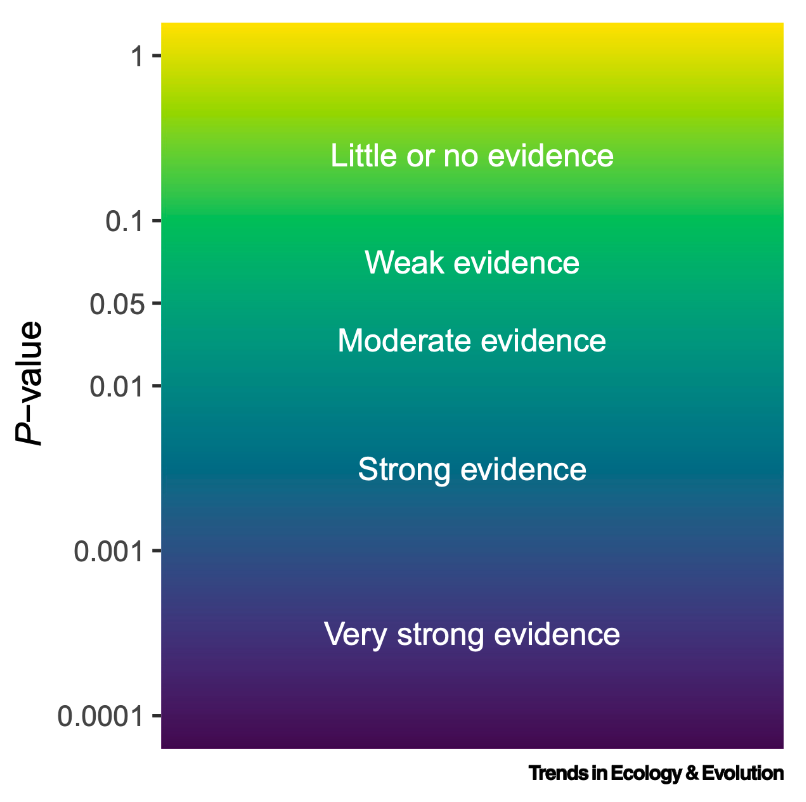
Because of the issues interpreting P-values, it is better to talk about what P-values tell you about the evidence for your hypothesis, rather than a strict idea of rejecting or not your hypothesis. Here is an illustration of how to interpret your P-values¹³:

(from Muff et al. (2022))

2.2 Limitations of P-values

As mentioned in the previous section, problems with the P-value method of testing your research hypothesis comes when you have more than one predictor in your hypothesis. Correlation among your predictors^¹⁴ means that it is difficult to trust your coefficient estimates. This means that you can not use the P-values as a way to determine which coefficients are significantly different than zero when you have correlated predictors. Said another way, your assessment of whether a predictor is useful in your model will be uncertain if you have correlated predictors. And correlated predictors are very common. For this reason, we will be hypothesis testing using model selection for the remainder of the handbook.

3 Hypothesis testing using model selection

An alternative method of testing your hypothesis is through model selection. This method is more robust to issues like predictor collinearity and can be generally applied regardless of the structure of your experiment or model.

3.1 What is model selection

Compare the following two models:

WtChange \(\sim \beta_1\cdot Prey + \beta_0 + error\)
WtChange \(\sim \beta_0 + error\)

Note that model 2 can be made by making the coefficient of Prey (\(\beta_1\)) equal to 0 (i.e. if the effect of Prey on WtChange was zero). If you determined which of these two models better fits your data, you will know if \(\beta_1\) is likely to be 0 and, thus, whether or not you have evidence that Prey can explain variation in WtChange.

3.2 How do you use hypothesis testing for model selection

The steps involved in testing your hypothesis using model selection is

form your candidate model set
fit and rank models in your candidate model set
choose your best-specified model(s)

Let’s walk through these now.

Form your candidate model set

Your candidate model set contains models with all possible predictor combinations¹⁵. So the candidate model set for WtChange \(\sim Prey + 1\) is:

WtChange \(\sim Prey + 1\)

WtChange \(\sim 1\)

Another example

Here is another example:

if your hypothesis is

\(Resp \sim Pred1 + Pred2 + Pred1:Pred2 + 1\)

your candidate model set is

\(Resp \sim Pred1 + Pred2 + Pred1:Pred2 + 1\)

\(Resp \sim Pred1 + Pred2 + 1\)

\(Resp \sim Pred1 + 1\)

\(Resp \sim Pred2 + 1\)

\(Resp \sim 1\)

Note that the more predictors you have in your model, the bigger your candidate model set.

Hopefully you are starting to see that the difference among models in the candidate model set can be described by setting the coefficient associated with a particular predictor to zero. In this way, fitting and comparing the models in your candidate model set is a way of assessing the evidence for your hypothesis. This method is more robust to issues like predictor collinearity because you are assessing the evidence for a predictor’s effect on your response when each predictor is in a model alone and when it is in a model with other predictors.

One last note about your candidate model set: you must remember the biology when you form your candidate model set. There may be a biological reason why a certain model must not be included in your candidate model set (i.e. a model that defies biological logic). These should be excluded from your candidate model set. (Burnham and Anderson (2002)).

Fit and rank models in your candidate model set

Next, each model in the candidate model set is fit to your data and graded based on an estimate of the model’s “cost” vs. its “benefit”.

The model’s cost is how many parameters the model has where you have preference for a simpler model (less parameters; see “The Principle of Parsimony” section below].

The model’s benefit is how well the model fits your data - i.e. how much of the variability in your response the model explains. The benefit estimate relates to the likelihood measure that was used to fit your model and estimate your coefficients (described in the Starting Model section).

The Principle of Parsimony

The principle of parsimony means that, when in doubt, you will choose the simpler explanation. This means that:

models should have as few parameters as possible
linear models are preferred to non-linear models
models with fewer assumptions are better

This said, there are times when you might choose a more complicated explanation over a simpler explanation. One example of this is when you prioritize a model’s ability to predict a future response vs. getting an accurate understanding of the underlying mechanisms (e.g. using a model to accurately predict tomorrow’s weather vs. understanding the mechanisms behind tomorrow’s weather). We will discuss this more in the upcoming section on Prediction.

You can fit and rank your models quickly using a function called dredge() in the MuMIn package¹⁶. The dredge() function fits and ranks models representing all possible predictor combinations based on your validated starting model - i.e. your default candidate model set¹⁷. The output is a table ranking the models in your candidate model set.

Let’s explore this now.

library(MuMIn) # load MuMIn package

options(na.action = "na.fail") # to avoid illegal model fitting

dredgeOut <- dredge(validMod) # create model selection table for validated starting model

print(dredgeOut)

Global model call: glm(formula = WtChange ~ Prey, family = gaussian(link = "identity"), 
    data = myDat)
---
Model selection table 
  (Intrc)    Prey df   logLik  AICc  delta weight
2  -6.996 0.07991  3  -29.864  66.1   0.00      1
1  -2.238          2 -125.489 255.2 189.07      0
Models ranked by AICc(x)

Note the line:

options(na.action = "na.fail") # to avoid illegal model fitting

This is included because you need to make sure the data used to fit every model in your candidate model set stays the same. This could be violated if you have missing values in some of your predictor columns. This options() statement makes sure your model selection is following the rules.

The output of the dredge() function gives us

the Global model call (our original hypothesis), and
a Model selection table

The Model selection table contains one row for each model in our candidate model set. Let’s explore this now:

Find the column called “(Intrc)”. This column tells us when the intercept is included in the model. If there is a number in that column, the associated model in your candidate model set (row) contains an intercept. Note that by default all models will contain an intercept¹⁸.

Find the column called “Prey”. This column tells us when the Prey predictor is in the model. Notice the first row contains a number in the Prey column, while the second row is blank. This means that Prey is a predictor in the model reported in the first row but is missing from the model in the second. Note also that a number is recorded in the Prey column, row 1 (0.0799). This is the coefficient associated with the Prey predictor. Since we have a normal error distribution assumption, this coefficient can be considered the slope of a line¹⁹. If the predictor was a categorical predictor (vs. numeric predictor), a “+” would appear in the Model selection table when the categorical predictor was in the model.

So, in our example above, the model in the first row contains an intercept and the Prey predictor - i.e. the first row is the model WtChange ~ Prey + 1. The model in the second row contains only an intercept - i.e. the second row is the model WtChange ~ 1.

The rest of the columns in the model selection table contain information that help us rank the models.

the “df” column reports the number of model coefficients. Models that are more complicated (e.g. more predictors) will have a higher df as they require more coefficients to fit. Models with more terms are more “costly”. In the first row (WtChange ~ Prey + 1), df is 3 because the model fitting estimates three coefficients: one for the effect of Prey on WtChange, one for the intercept, and, since this is a normal error distribution assumption, one for the standard deviation. In the second row (WtChange ~ 1), df is 2 because the model fitting estimates a coefficient for the intercept, and for the normal error distribution assumption’s standard deviation. So the model in the first row is more “costly” than the second row.
the “logLik” column reports the log-Likelihood of the model fit. The absolute value of this estimate will depend on the type of data you are modelling, but in general, the logLik is related to how much variation in your response the model explains. It can be used to compare models fit to the same data. This can be seen as a measure of the “benefit” of the model.
the “AICc” column reports information criteria for your models. Information criteria balances the cost (complexity) and benefit (explained variation) for your model. An example of information criterion is the Akaike Information Criterion (AIC). The AIC is estimated as:

\(AIC = 2\cdot k - 2 \cdot ln(L)\)

where \(k\) is the cost of the model (number of coefficients, like df above), and \(L\) is the maximum likelihood estimate made when the model was fit (like logLik above).

There are other types of information criteria such as Bayesian Information Criteria (BIC, where the cost is penalized harsher, favouring a simpler model), and the corrected Akaike Information Criterion (AICc, where the metric is optimized for small sample sizes). The AICc is reported by default here, but you can control that in the dredge() function. In all cases, lower information criterion means more support for the model.

the “delta” (\(\Delta\)) column is a convenient way to see how different each model’s AICc is from the model with the lowest AICc (\(\Delta AIC_i\) is the change in AIC for model i vs. the model with the lowest AIC.)
the “weight” column reports Akaike weights for the model. The Akaike weights are a measure of the relative likelihood of the models. The sum of all the Akaike weights is 1, so we can get a relative estimate for the support for each model.

Akaike weights

Here is the equation to estimate the Akaike weights:

\[ w_i = \frac{exp(-\frac{1}{2} \cdot \Delta AIC_i)}{\sum_{r=1}^{R}exp(-\frac{1}{2} \cdot \Delta AIC_r)} \]

where

\(w_i\) is the Akaike weight for model i,
\(\Delta AIC_i\) is the change in AIC for model i vs. the model with the lowest AIC
\(\Delta AIC_r\) is the change in AIC for model r vs. the model with the lowest AIC. This is estimated for all models in the candidate model set (R models).

Burnham and Anderson (2002)

Choose your best-specified model(s)

Using the model selection table, you can choose your best-specified model(s) and find out what it tells you about your hypothesis.

In general, your best-specified model will be the model with the lowest information criterion (e.g. AIC)²⁰. This will be the model at the top of the model selection table.

That said, notice I write “best-specified model(s)” - possibly plural. This is because you might have models where the AIC estimates are very close to one another. A good rule of thumb is to report all models where the AIC is within 2 of the lowest AIC model (i.e. delta < 2). Following Burnham and Anderson (2002),

for models where delta is	there is … for the model
0-2	substantial support
4-7	considerably less support
> 10	essentially no support

Remember that ambivalence about which is the best model to explain variability in your response is a valid scientific result (Burnham and Anderson 2002). Report all possible best-specified models and discuss what they mean for your research hypothesis and area, including possible follow-up studies that could be done to further the science in this area. More on this is discussed in the section on Communicating.

With our example above:

print(dredgeOut)

Global model call: glm(formula = WtChange ~ Prey, family = gaussian(link = "identity"), 
    data = myDat)
---
Model selection table 
  (Intrc)    Prey df   logLik  AICc  delta weight
2  -6.996 0.07991  3  -29.864  66.1   0.00      1
1  -2.238          2 -125.489 255.2 189.07      0
Models ranked by AICc(x)

we have one best-specified model (model with substantial support):

WtChange ~ Prey + 1 (AICc = 66.1)

and essentially no support for the null model:

WtChange ~ 1 (AICc = 255.2; delta = 189.1)

We can conclude that there is evidence that Prey explains variability in WtChange.

What does your best-specified model(s) say about your hypothesis?

Model selection is a way of hypothesis testing. So what does your best-specified model say about your hypothesis? By comparing your best-specified model to your validated starting model, you can see where there is evidence for the effects of each predictor, and where the effects are estimated to be zero.

As our best-specified model is

WtChange ~ Prey + 1

We can conclude that there is evidence that Prey explains variability in WtChange.

More examples

if our validated starting hypothesis was:

\(Resp \sim Pred1 + Pred2 + Pred1:Pred2 + 1\)

A best-specified model of \(Resp \sim Pred1 + Pred2 + Pred1:Pred2 + 1\) would indicate that we have evidence that there are effects of Pred1 and Pred2 on Resp and that the effect of Pred1 on Resp depends on Pred2 (an interaction).
A best-specified model of \(Resp \sim Pred1 + Pred2 + 1\) would indicate that we have evidence that there are effects of Pred1 and Pred2 on Resp but no evidence of an interaction effect.
A best-specified model of \(Resp \sim Pred1 + 1\) would indicate that we have evidence that there is an effect of Pred1 but not Pred2 on Resp.
A best-specified model of \(Resp \sim 1\) (i.e. the null hypothesis) would indicate that we have no evidence for effects of Pred1 or Pred2 on Resp. This is also a valid scientific result!

In the next section (on Reporting), we will discuss further how to communicate what your hypothesis testing results say about your hypothesis.

References

Burnham, K. P., and D. R. Anderson. 2002. Model Selection and Multimodel Inference: A Practical Information-Theoretic Approach. Springer Verlag.

Muff, Stefanie, Erlend B. Nilsen, Robert B. O’Hara, and Chloé R. Nater. 2022. “Rewriting Results Sections in the Language of Evidence.” Trends in Ecology &Amp; Evolution 37 (3): 203–10. https://doi.org/10.1016/j.tree.2021.10.009.

Popovic, Gordana, Tanya Jane Mason, Szymon Marian Drobniak, Tiago André Marques, Joanne Potts, Rocío Joo, Res Altwegg, et al. 2024. “Four Principles for Improved Statistical Ecology.” Methods in Ecology and Evolution 15 (2): 266–81. https://doi.org/10.1111/2041-210x.14270.

Footnotes

inference is the conclusion you make based on reasoning and evidence↩︎
vs. categorical↩︎
if you are confused why we are choosing these assumptions, read the Starting Model section again↩︎
these estimates are called parameters↩︎
others not discussed here include cross-validation, Bayes Factors, confidence intervals↩︎
note that some write this as “P value” and some as “p value” and some as “p-value”. There is no one rule. Just pick one and make it consistent through your text. We will try to do that here.↩︎
field↩︎
see more in the section on Data curation and collection ↩︎
see more in the section on Model Validation ↩︎
because it is generally applicable↩︎
i.e. the effect of Prey on WtChange↩︎
for example, a P value of 0.006 means that there is a 0.6% chance we would estimate the effect of Prey to be 0.12 \(g \cdot m^{3}\cdot num{-1}\) when it was in fact 0↩︎
we’ll come back to this in the Reporting section↩︎
see more in the section on Model Validation ↩︎
these are also called “nested” models as each model is “nested” in one of the other models when it only differs by one predictor. “Nested” is also used in experimental design to mean something totally different, so we will avoid using the term here.↩︎
note the spelling and capitalization of this package name!↩︎
other methods include forwards or backwards model selection. In these, you add (or subtract) one predictor term from your starting model to determine the effect on your model’s ability to explain the variability in your response. These methods can be biased by collinearity among your predictors in your model, so we will proceed with looking at all possible predictor combinations as described here↩︎
indeed, your null model only contains an intercept↩︎
and it is the same number given in the summary() output above. More on this coming up in the Reporting section!↩︎
Note that lower is always better with information criterion, though the magnitude of the AIC value will change from case to case.↩︎