how to determine if your starting model can be used to test your hypothesis
what to do if your model is mis-specified
1 Validating your starting model
1.1 Why do you need to validate your starting model?
As we discussed before “All models are wrong, but some are useful”. So how do you tell if your starting model is a useful one; that is, one that can be used to test your hypothesis?
When you choose your starting model you make an educated guess as to what a useful starting model might be, but you can only validate that it is a useful starting model after you have fit the model to your data.
A useful model is one that reflects the mechanistic understanding of your research hypothesis (the deterministic part of your model - your shape assumption) as well as the nature of your observations (the stochastic part of your model - your error distribution assumption)1.
In addition, a useful model is one that conforms to the assumptions of the method you use to test your model (e.g. GLM). The assumptions of the GLM include that your predictors are not correlated with one another, and that your observations are independent of one another.
In this section, we will explore each of these assumptions by considering if your:
By considering these four points, you can determine if your model is “well-specified” to test your hypothesis.
In this section, we will go over tools that will help you determine if your model is well-specified and what to do if you find yourself with a mis-specified starting model (e.g. updating your starting model).
“A well-specified model”
Note that you are trying to find “a well-specified model”. This terminology reflects the fact that more than one model2 is likely appropriate to test your hypothesis.
2 A statistical modelling example
It will help our discussions to have an example of a starting model. For our example, consider the research hypothesis that your response variable Resp is explained by a categorical predictor (Cat), two continuous predictors (Cont1 and Cont2) as well as the interactions among all predictors. You communicate this as:
In this example, Resp is a positive, continuous variable.
Let us assume you tested this hypothesis by fitting a model with a Gamma error distribution assumption (to reflect the nature of your response variable) and linear shape assumption (to reflect the relationship between each predictor and your response, assuming in all cases these are linear) using a GLM:
startMod<-glm(formula = Resp ~ Cat + Cont1 + Cont2 + Cat:Cont1 + Cat:Cont2 + Cont1:Cont2 + Cat:Cont1:Cont2 +1, # hypothesisdata = myDat, # datafamily =Gamma(link="inverse")) # error distribution assumptionsummary(startMod) # a look into our model object
Call:
glm(formula = Resp ~ Cat + Cont1 + Cont2 + Cat:Cont1 + Cat:Cont2 +
    Cont1:Cont2 + Cat:Cont1:Cont2 + 1, family = Gamma(link = "inverse"),
    data = myDat)

Coefficients:
                           Estimate Std. Error t value Pr(>|t|)
(Intercept)               1.363e-01  1.827e-02   7.461 3.41e-12 ***
CatTreatment             -4.921e-02  2.150e-02  -2.288 0.023260 *
Cont1                    -1.514e-03  3.843e-04  -3.940 0.000116 ***
Cont2                    -2.615e-03  1.419e-03  -1.843 0.066977 .
CatTreatment:Cont1        4.181e-04  4.515e-04   0.926 0.355643
CatTreatment:Cont2        1.385e-03  1.657e-03   0.835 0.404560
Cont1:Cont2               4.637e-05  2.520e-05   1.840 0.067390 .
CatTreatment:Cont1:Cont2 -2.089e-05  2.978e-05  -0.701 0.483944
---
Signif. codes:  0 '***' 0.001 '**' 0.01 '*' 0.05 '.' 0.1 ' ' 1

(Dispersion parameter for Gamma family taken to be 0.02183205)

    Null deviance: 24.1090  on 189  degrees of freedom
Residual deviance:  4.0425  on 182  degrees of freedom
AIC: 994.32

Number of Fisher Scoring iterations: 4
We will consider this model as we proceed through this section.
3 Considering predictor collinearity
What it is:
NOTE: predictor collinearity3 is only a problem if you have more than one predictor in your hypothesis.
Your model assumes that your predictors are not correlated with one another, and that each predictor explains a unique part of the variation in your response. When this assumption is violated, the estimates of the coefficients4 become more uncertain and you are unable to test your hypothesis in a robust way.
Let us use an extreme case to see why this might be a problem:
Imagine you are interested in explaining variability in plant growth (your response is plant growth). You think temperature and water may influence plant growth, so you set up an experiment where you will grow plants under high and low temperature and high and low water (your predictors are temperature and water treatments). But in your experimental set-up you only include two treatments: one where the plants are grown with high temperature and high water, and another where plants are grown with low temperature and low water. In your experiment, your predictors are correlated with one another5. When you try to test your hypothesis, you will not be able to say if the growth differences between treatments are due to differences in temperature or water.
This is an extreme case (where your predictors are 100% correlated with one another), and one that can easily be avoided with a better experimental design. But, predictors that are at least partially correlated with one another are very common in observational/field studies (e.g. things like salinity, temperature and depth in marine studies).
Predictor collinearity causes a problem with our interpretation of our model because it increases the error around the coefficients (modelled effects). This error can be so large, that we are unable to assess the effect of a predictor in explaining the response. This increase in error due to predictor collinearity is called “variance inflation”6. This is a problem for your statistical modelling (as it becomes difficult to quantify the predictor effects in your model) and for your work as a biologist (as you are unable to mechanistically explain the variability in your response).
How you know if you have a problem:
You may have a hunch that you will have a problem with predictor collinearity before you even fit a model. You can identify potential problems by looking at correlations of your predictors with one another.
Here is a helpful bit of code for your investigations, applied to our example model:
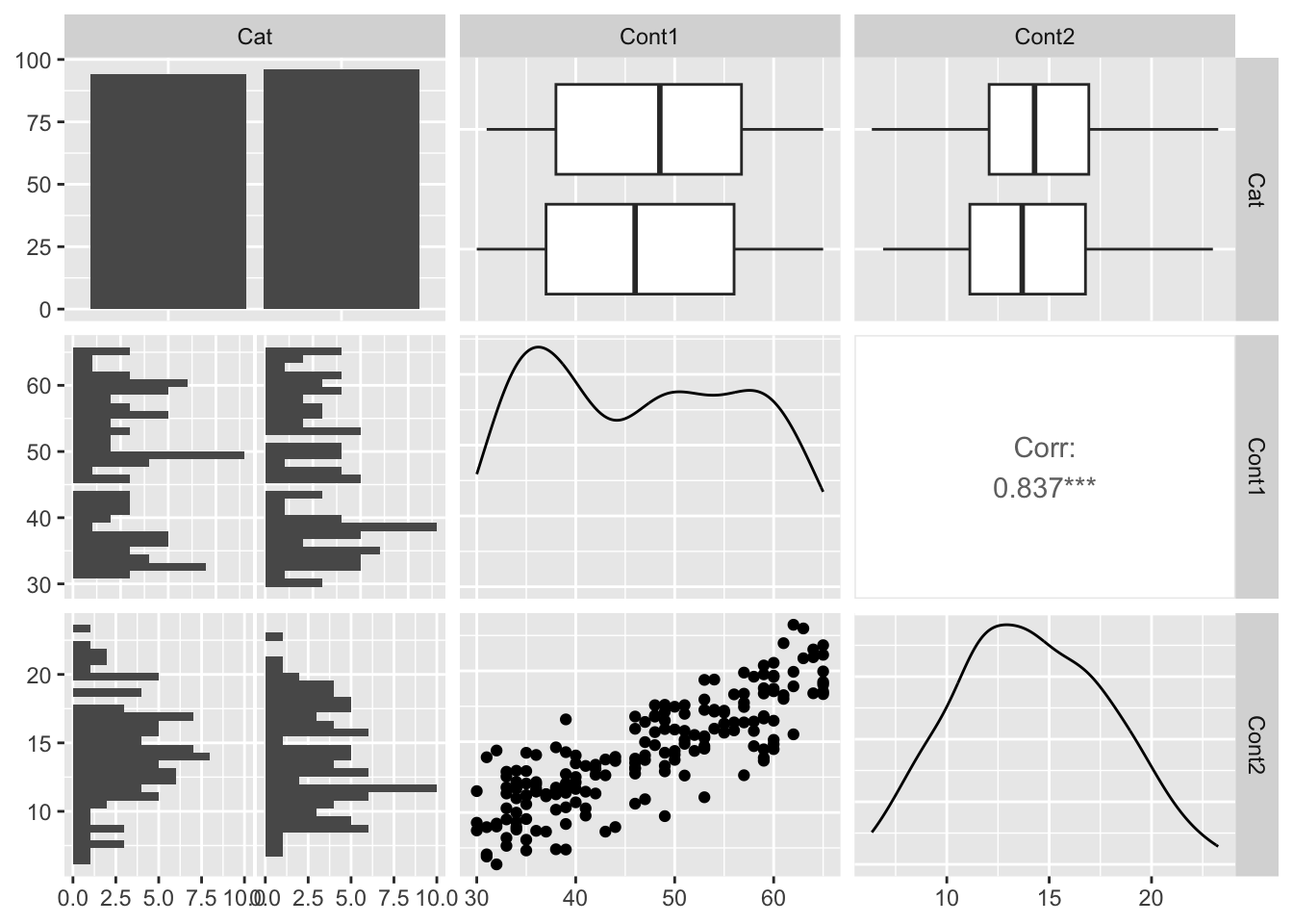
library(dplyr) # loading the dpllyr package, for select() functionmyPreds <-select(myDat, Cat, Cont1, Cont2) # make a data frame with only my predictor columnslibrary(GGally) # loading GGally package, for ggpairs() functionggpairs(data = myPreds) # make a plot of your predictors - each column vs. another - often called a "pairs plot"
Note in the figure above that there is a linear pattern in the Cont1 vs. Cont2 plot, and that there is a correlation estimate of 0.84 for this predictor pair. This indicates predictor collinearity, and that having both Cont1 and Cont2 in your model may result in variance inflation.
You can also see how much of a problem predictor collinearity is causing by estimating variance inflation factors (VIFs) after you fit your starting model. VIFs look at your model to see how much correlation among predictors is making your coefficient estimates uncertain.7
In general, when a VIF is greater than 3 (or adjusted GVIF8 is greater than \(\sqrt 3\)), predictor collinearity is a cause of concern. When VIF is greater than 5 or 10 (or adjusted GVIF9 is greater than \(\sqrt 5\) or \(\sqrt 10\)) the influence of predictor collinearity on your coefficients is enough that you need to take action (Fox and Monette 1992). For this handbook, we will use the more conservative threshold of VIF > 3 (or adjusted GVIF10 > \(\sqrt 3\)) as our criterion.
Generalized variance inflation factors (GVIF)
Note that when you have a categorical predictor that has more than two categories (levels), VIFs need to be calculated in a different way - as generalized VIFs (or GVIFs).
This is due to how R fits models with categorical predictors. R does this by modelling the difference in the response when moving from one categorical level to another (a reference level). You want the VIF results to be independent of which level R chooses as its reference level - this is what GVIFs do.
You can use the same function vif() from the car package to estimate both VIFs and GVIFs. The function will choose the appropriate equation for you based on your model.More on this below.
Note that the threshold for when we would consider VIF as being a problem is greater than 3 for traditional VIFs and greater than \(\sqrt 3\) for GVIFs.
You can limit the risk of predictor collinearity by carefully planning your experiments to limit predictor correlation as much as possible. If you identify a problem with collinearity, you can:
remove one or more of the offending predictors to remove the problem. Note that removing a predictor will change your research hypothesis.
keep the predictor(s) in but be careful when you interpret the effects estimated by your model.11
library(car) # load the car packagevif(startMod.noInt) # estimate VIFs
     Cat    Cont1    Cont2
1.007510 3.341182 3.354825
Note that there are two VIF values higher than the threshold value (in this case VIFs > 3). This means that the presence of both Cont1 and Cont2 in the model is resulting in variance inflation.
Let us remove one of the predictors (Cont2)13 and recalculate the VIFs:
## Recalculating the VIFsvif(startMod.noInt.noCont2) # estimate VIFs
     Cat    Cont1
1.002028 1.002028
There are no longer major problems with predictor collinearity as all VIFs < 3. Let us refit this as our starting model, and recalculate the residuals (as we will need them soon):
## Refitting your starting model with the interactions back in:startMod <-glm(formula = Resp ~ Cat + Cont1 + Cat:Cont1 +1, # hypothesisdata = myDat, # datafamily =Gamma(link ="log")) # error distribution assumptionsummary(startMod) # a look at the model object
Call:
glm(formula = Resp ~ Cat + Cont1 + Cat:Cont1 + 1, family = Gamma(link = "log"),
    data = myDat)

Coefficients:
                   Estimate Std. Error t value Pr(>|t|)
(Intercept)        2.073821   0.071662  28.939  < 2e-16 ***
CatTreatment       0.275824   0.098617   2.797  0.00570 **
Cont1              0.015891   0.001480  10.740  < 2e-16 ***
CatTreatment:Cont1 0.005387   0.002053   2.624  0.00942 **
---
Signif. codes:  0 '***' 0.001 '**' 0.01 '*' 0.05 '.' 0.1 ' ' 1

(Dispersion parameter for Gamma family taken to be 0.02151095)

    Null deviance: 24.1090  on 189  degrees of freedom
Residual deviance:  4.0505  on 186  degrees of freedom
AIC: 986.69

Number of Fisher Scoring iterations: 4
Our starting model has now past the first hurdle to being considered wellspecified: no (significant) predictor collinearity.
4 The role of residuals in validating your model
As a reminder, you are validating your model considering four assumptions:
Validating assumptions 2 through 4 require you to consider the residuals of your model fit.
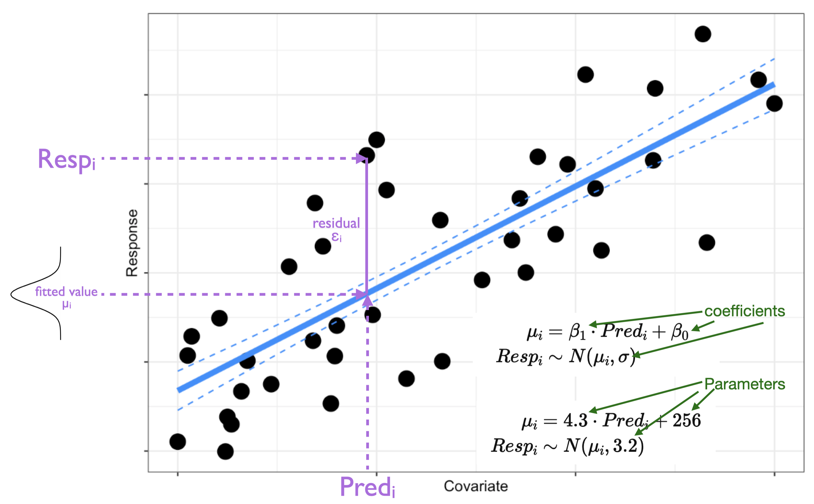
Recall that a residual can be defined as14 the difference between the model fitted value and your response observation:
When your model is a useful one (a valid one for testing your hypothesis), these residuals will:
follow the expected error distribution assumption, and
be constantly distributed relative to your model fit and each of your predictors, and
be constantly distributed relative to variables NOT in your model.
In fact, you can only validate the assumptions you made when picking your starting model after the model is fit because violations show up in the model residuals.
We will be looking at two types of plots to help us investigate the model residuals.
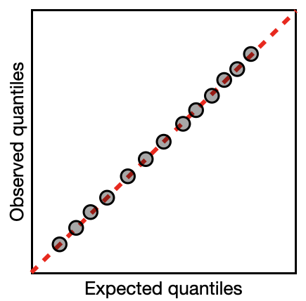
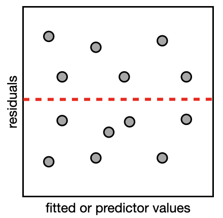
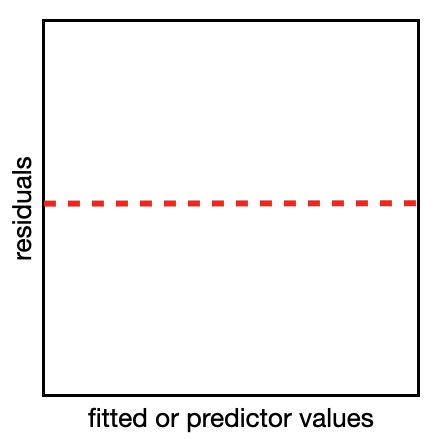
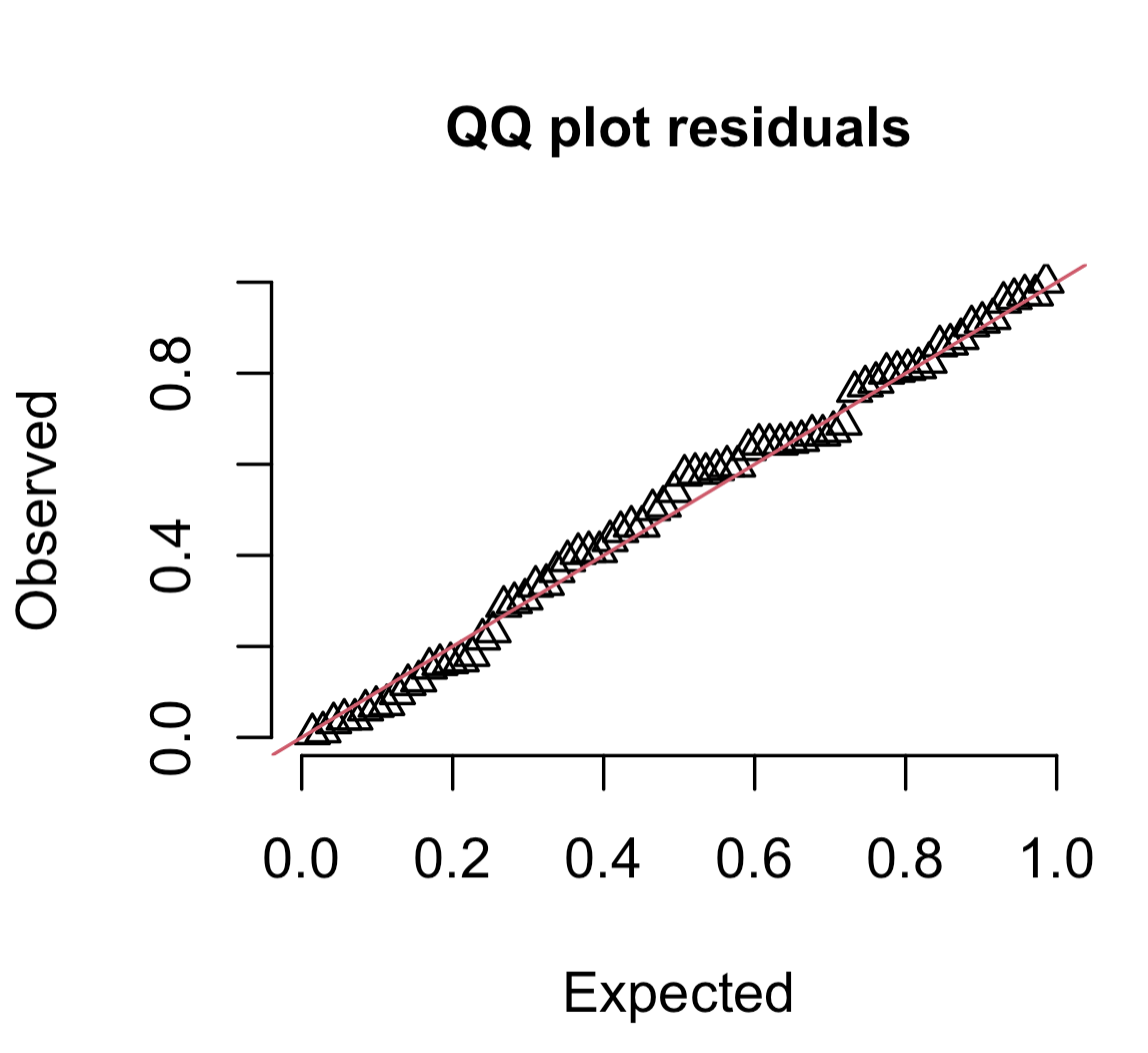
The first is a quantile-quantile (QQ) plot. A reminder from the section on Data Distributions that a quantile breaks your observations into groups, e.g. the 25% quantile is the value of the variable where 25% of the values are below this value. A quantile-quantile plot compares the position of the quantiles in the expected and observed residual distribution to see if they come from the same distribution. If they come from the same distribution, the quantiles will match, the points will lie along a 1:1 (red) line on the QQ plot, and your model assumption is valid (like the example on the right).
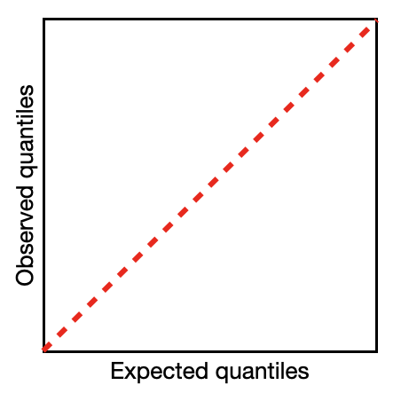
The second type of plot is a residual plot. In the residual plot, you will make plots to compare the residuals (on the y-axis) vs. the model fit and each predictor/variable (on the x-axis). This will let you see if there are any patterns in the plot which could indicate a violation of your model assumptions. If your model is valid, the points will form a uniform cloud of points in your residual plot (like the example on the right).
You have been looking at residuals as simple differences between your model fit and the observation of your response (as pictured above). The information that you can get from this type of residual will vary with the structure of your model… this can make residual inspection frustrating, as you would have to learn a new method of considering your residuals for each new type of model (Hartig 2024).
Instead, you will be using a particular type of residual to validate your starting model - one that can be interpreted in similar ways whatever your model structure. It is called a scaled residual.
4.1 A useful residual - the scaled residual
As mentioned above, inspecting scaled residuals gives us a method of validating our model that is generally applicable - GREAT - but it also is a method that is intuitive: The scaled residual method checks to see if your model is useful (valid) by seeing if it can even produce data that looks like the data you used to fit your model (i.e. your observations). A model that is well-specified will be able to simulate data that looks like the data used to fit it.
We will estimate and explore scaled residuals using functions in the DHARMa package.
DHARMa’s scaled residuals
The DHARMa package uses a simulation-based approach15 to estimate scaled residuals. These scaled residuals are standardized to a uniform distribution regardless of the model structure.
Here’s how it works:
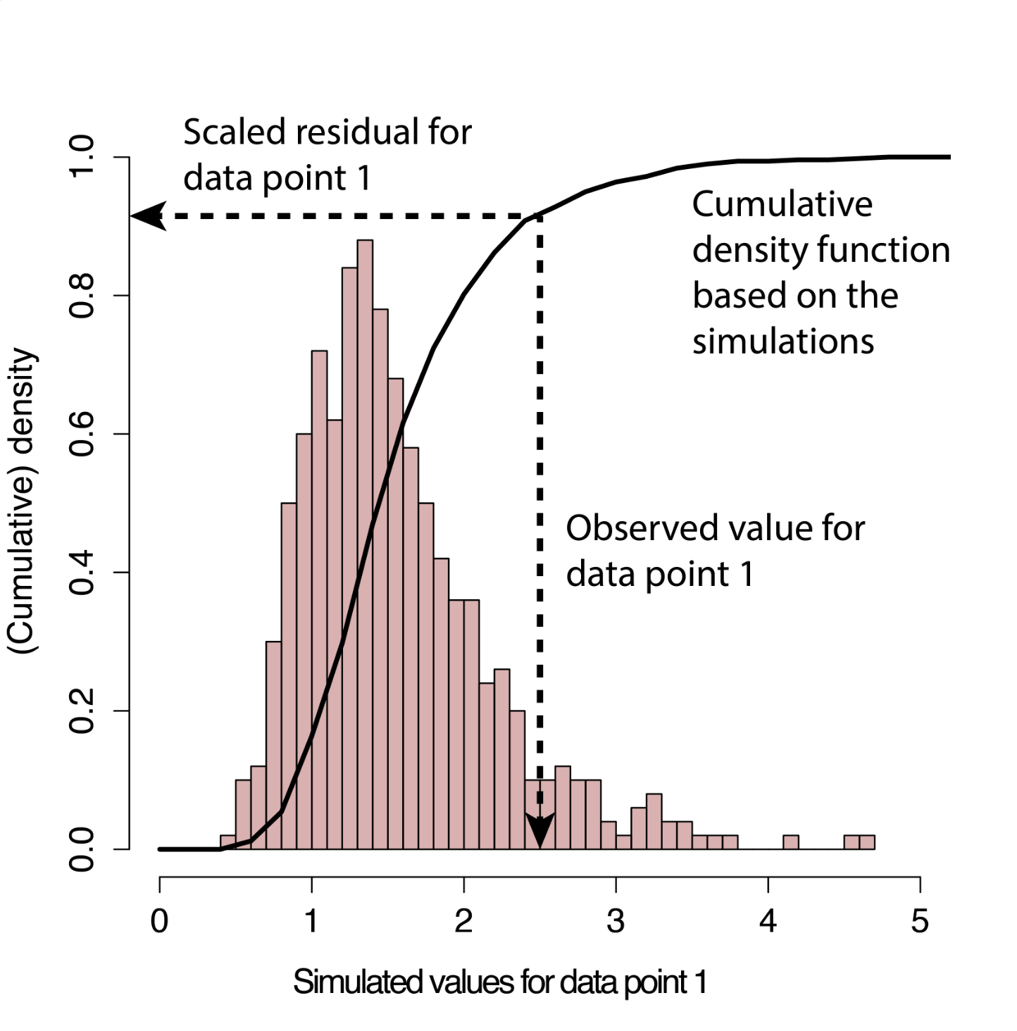
DHARMa uses your starting model to simulate new response data for each observation (each row in your data frame). The default is that it simulates 250 new data sets from your model16.
DHARMa uses the simulated values at each observation to calculate the empirical cumulative density function (ECDF) of the simulated values at that observation.
The scaled residual for observed data point i is then defined as the value of the ECDF at the value of the observed data i (see figure to the right).
Estimated this way, if your model is well-specified, the scaled residuals will always follow a uniform distribution, regardless of your starting model structure. Put another way: if the observed data were created from the same data-generating process of your starting model, all values of the cumulative distribution should appear with equal probability and the DHARMa residuals will be distributed uniformly.
Note: because DHARMa simulates new data each time it is run, you can get variability in your results from run to run. To avoid this, you can use the function set.seed() which is used to set the seed for the random number generator R is using to simulate the data. This gives the random number generator a specific starting point, so the random numbers (and simulated residuals) are reproducible.
Let us estimate the residuals from our example starting model using the scaled residual method mentioned above.
library(DHARMa) # load packagesimOut <-simulateResiduals(fittedModel = startMod, n =250) # simulate data from our model n times and calculate residualsmyDat$Resid <- simOut$scaledResiduals # add residuals to data framestr(myDat) # check the structure of the data
The residuals have been added to the data frame as myDat$Resid. We will take a look at these residuals as we walk through the model validation below for the remaining three assumptions:
In case useful in your future work, alternatives to the methods described here are:
the performance package where you can get residuals and diagnostic plots with the check_model() function.
the car package where you can get a sense for how well your model is capturing the features of your data using the marginalModelPlots() function.
5 Considering observation independence
What it is:
Many model fitting methods (including GLMs) assume that the individual observations (e.g. each row in your data frame) are independent from one another. This means that the observations are not correlated (grouped) with one another in any way except as described in the predictors in your hypothesis. If this is true, each individual observation (row) can be called a replicate. When this assumption is violated, and you have observation dependence, it makes the estimate of your coefficients inaccurate, limiting the usefulness of your model.
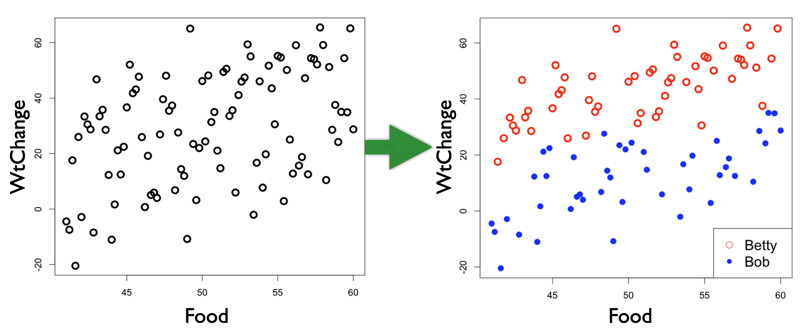
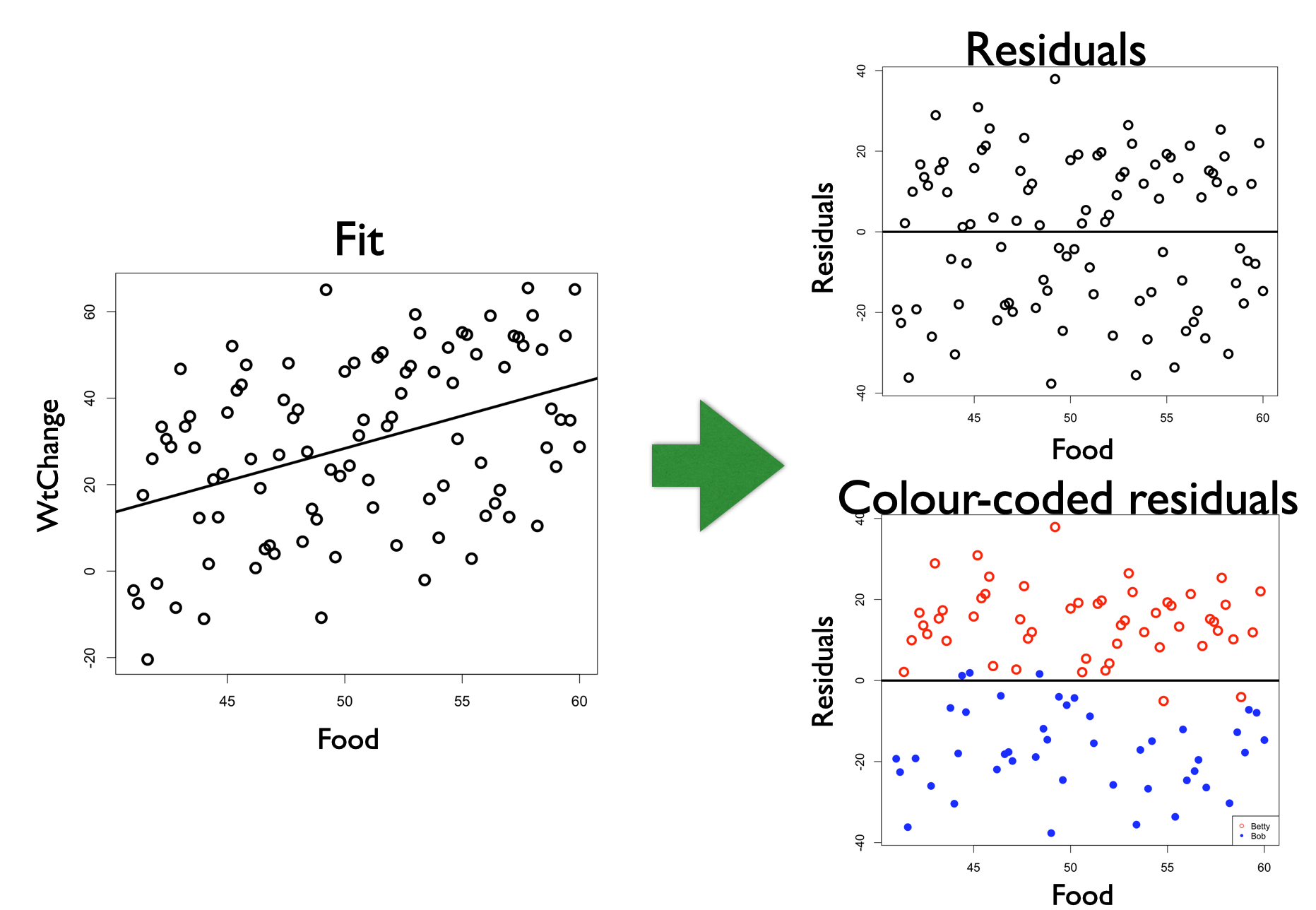
Here is an example where you want to test the hypothesis that weight change is explained by food consumption (WtChange ~ Food);
Notice that Observer is not in your research hypothesis, but it is structuring your observations - the observations sampled by Betty are more similar than those sampled by Bob. Without information about Observer, you will have a difficult time fitting the model to your data. Without the information about Observer, the “noise” of unexplained variation is high compared to the “signal” of the effect of Food on WtChange.17. This is a problem for your statistical modelling and work as a biologists as effects will be difficult to identify in your hypothesis testing.
How you know if you have a problem:
An easy way to tell if you have a problem is to plot your model residuals vs. any variable you suspect as being a source of dependence among your observations. For example, highlighting Observer in the residuals with the example above:
If Observer had no effect on WtChange, we would see no pattern in the colours of the residuals when plotted vs. Observer, but, instead, we see the colour of the residual points grouping together. If you have a dependence problem in your model, you will see the “structure” in the unexplained variability (residuals).
5.1 Types of observation dependence and what you can do about them
It is relatively common to find violations of this assumption18. Violations can happen from:
grouping of your observations by a variable not in your hypothesis (as the example above)19
observations that are made at different times (temporal autocorrelation)
observations that are made at different locations (spatial autocorrelation)
Grouping - a missing predictor
Grouping occurs when you have observations dependent on one another due to some other variable not in your hypothesis. This may be a site variable (e.g. garden plots), or a variable that impacts your measurement (e.g. observer, or gear type), or could be related to repeated measurements (e.g. sampling the same individual multiple times).
An example
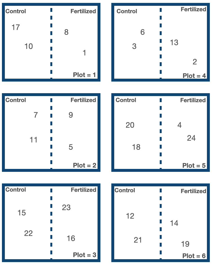
Another example: you might be exploring the effect of added fertilizer on plant height with your hypothesis being Height ~ Fertilizer, with Fertilizer being a categorical predictor with levels of “Fertilized” or “Control”. In making your observations, you measure 24 plant heights growing in a Fertilized or Control site. Oh, and these sites happened to be organized across six experimental plots.
Given your hypothesis that Height ~ Fertilizer, each measurement of plant height will be treated as an individual observation (replicate) with the assumption that, other than the Fertilizer treatment, these observations are independent of one another. However, this assumption is violated as the plants from the same plots may be more similar than plants from different plots (e.g. sunlight differences across plots may influence plant height, or water drainage differences across plots may influence the effect of the fertilizer). For example, plant IDs 17, 10, 8 and 1 may be more similar to one another than other plants in the experiment because they are all growing from Plot #1. The Plot variable may be grouping your observations.
How you know if you have a problem with observations dependent based on a grouping variable
You can find out if observation dependence is influencing your model by inspecting the residuals of your starting model. Here, you plot your residuals vs. variables not in your model that may be causing dependence in the observations.
If you have a problem with observation dependence, there will be a pattern in your residuals when plotted against the offending variable.
If there is no problem with observation dependence, there will be no pattern in your residuals.
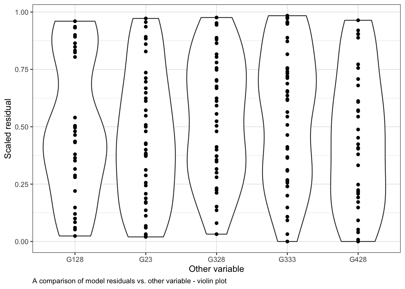
Here is an example of how to do this with our generic example started above. You can see how the residuals differ across levels of the Other variable also in our data set using violin plots:
ggplot()+# start ggplotgeom_violin(data = myDat,mapping =aes(x = Other, y = Resid))+# add observations as a violingeom_point(data = myDat,mapping =aes(x = Other, y = Resid))+# add observations as pointsxlab("Other variable")+# y-axis labelylab("Scaled residual")+# x-axis labellabs(caption ="A comparison of model residuals vs. other variable - violin plot")+# figure captiontheme_bw()+# change theme of plottheme(plot.caption =element_text(hjust=0)) # move figure legend (caption) to left alignment. Use hjust = 0.5 to align in the center.
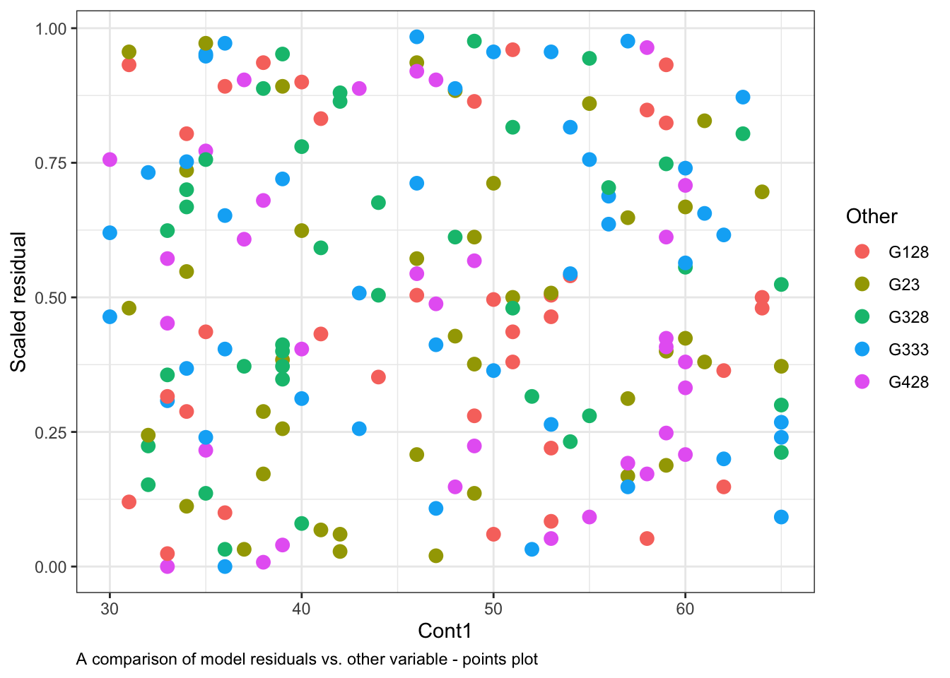
or with a points plot, by colouring the residuals based on the level in Other20:
ggplot()+# start ggplotgeom_point(data = myDat, # the data framemapping =aes(x = Cont1, y = Resid, col = Other), # add observations as pointssize =3)+# change the size of the pointsxlab("Cont1")+# y-axis labelylab("Scaled residual")+# x-axis labellabs(caption ="A comparison of model residuals vs. other variable - points plot")+# figure captiontheme_bw()+# change theme of plottheme(plot.caption =element_text(hjust=0)) # move figure legend (caption) to left alignment. Use hjust = 0.5 to align in the center.
Note that the spread of the residuals in each level (category) of Other is fairly equal in the violin plots and the colours are spread across the points plot. This indicates that Other variable is not causing much structure in the residuals, and likely is not causing the model to violate the assumption of independence.
Finally, if you quantitative evidence that your observations are dependent on your grouping variable, you can test to see if residuals among the different groups have similar variances. This can be done with a Levene test for the homogeneity of variances through functions in the DHARMa package, e.g.
library(DHARMa) # load packagetestCategorical(simOut, # the residuals catPred = myDat$Other)$homogeneity # the grouping variable of concern
Levene's Test for Homogeneity of Variance (center = median)
       Df F value Pr(>F)
group   4  0.1112 0.9785
      185
plotResiduals(simulationOutput = simOut, # compare simulated data to form = myDat$Other, # our observationsasFactor =TRUE) # whether the variable plotted is a factor
When your P-value is large (as it is here: P = 0.978), you would say that there is no evidence that the residual variance depends on the levels in Other (i.e. no concern for observations being dependent on Other).
What can you do if your observations are grouped by something not in your hypothesis
If you find evidence of observation dependence, you can:
Treat an offending group as an outlier: If you have one group causing structure in your residuals, you can try removing the group (documenting that you have done so) and proceed with your modelling. Remember to be transparent that you have done this, in the Results and Discussion, including spending some time (and sentences) contemplating why the group might be behaving differently.
Add the grouping variable to your model as a (fixed effect) predictor: The assumption of observation independence means that your observations are independent of one another in all ways except for the predictors already included in your hypothesis. Therefore, an easy way to address observation dependence is to include the variable in your hypothesis, e.g. changing your original model:
Height ~ Fertilizer + 1
to
Height ~ Fertilizer + Plot + Fertilizer:Plot + 1
would account for variability in plant height that was due to the plants growing in different plots (the main effect of Plot), as well as the influence of plot on the effect fertilizer has on the plants (the interaction Fertilizer:Plot).
Note that adding Plot in this way is adding Plot as a “fixed effect” (vs. “random effect” - more on this below). In fact, every predictor we have been discussing up until now is in our model as something called a fixed effect.
A couple of things to note when you add new fixed effects to your model:
Fixed effects influence the mean of the model prediction, and so they are formerly part of your research hypothesis. This means that your hypothesis changes every time you add or remove a fixed effect. Your original hypothesis was
Height ~ Fertilizer + 1
or that variability in plant height is explained by fertilizer addition. If you add Plot to your hypothesis to deal with observation dependence, your research hypothesis becomes:
Height ~ Fertilizer + Plot + Fertilizer:Plot + 1
or that variability in plant height is explained by fertilizer addition, plot ID and the interaction between the two.
When you add new fixed effects to your hypothesis, your model gets more “expensive” to fit. In the section on Hypothesis Testing, we will discuss how we can quantify the “benefit” of the model (increased explained deviance related to the likelihood of the model) vs. the cost of the model (how many coefficients have to be estimated to fit your model). Adding new fixed effects increases the cost of fitting your model as more coefficients need to be estimated. This increased cost means you need more observations (data) to fit the model. When you add a new continuous predictor to your hypothesis, there is one more coefficient to estimate (in a linear model, this is a slope). When you add a new categorical predictor to your hypothesis, you need to estimate another coefficient for each level in your new predictor. In our example, you would need to estimate 6 - 1 = 521 new coefficients to add the main effect of the Plot variable to the model, and another 6 - 1 = 5 coefficients to add the Fertilizer:Plot interaction to the model.
Both points above (that your hypothesis will change, and that your model will be more expensive to fit) means that just adding your grouping variable to deal with observation dependence is not always a great option. Instead you could,
Add the grouping variable to your model as a random effect using a mixed model: Many turn to mixed modelling as a way to deal with observation dependence. Mixed modelling22 is called “mixed” modelling because it includes a mix of both fixed effects (predictors that influence the model predicted mean) and random effects (predictors that influence the model predicted variance). Fitting mixed models will be covered in an upcoming handbook section, but I wanted you to have an idea of what mixed modelling is, and how to get started with mixed modelling, in case you want to use these methods in the future.
To fit mixed models in R, you need to adjust your hypothesis formula to tell R which predictors should be treated as fixed and which should be random. Recall that your model with only fixed effects:
Height ~ Fertilizer + Plot + Fertilizer:Plot + 1
indicates that the predicted mean height is affected by fertilizer, plot ID and the interaction between the two, with separate coefficients associated with each plot ID. In mixed modelling, you could instead include Plot with:
The (1|Plot) term will estimate one (not 5) extra coefficient describing how the variance in average height (the intercept) varies when you move from plot to plot. The (Fertilizer|Plot) term will estimate one (not 5) extra coefficient describing how the variance in the effect of the fertilizer varies by plot.
So mixed modelling offers a way to address dependence in your observations that does not change your research hypothesis (as you are not adding fixed effects) and is cheaper (requiring less coefficient estimates as the random effects influence the modelled variance, not the mean).
You can fit mixed models in the lme4 package using the glmer() function (which stands for Generalized Linear Mixed Effects Models, or GLMM), with syntax that is very similar to what we have been using for GLMs, e.g.
One final thing to note is that random effects will always be categorical. If you have a continuous variable that is causing dependence in your observations, this variable can not be included as a random effect and must be included as a fixed effect.
Here is a table if you are trying to determine if a variable causing dependence in your model should be included as a fixed or random effect:
Your situation
Your choice
- the variable causing dependence is continuous - if you are interested in effect sizes of the variable on your response - if the factor levels are informative (vs. just numeric labels)
fixed effect
- the levels in the variable are only samples from a population of levels - if you have enough levels (at least 5) to estimate the variance of the effect due to your variable23
random effect
(adapted from Crawley2013TheRBook)
Temporal autocorrelation
Temporal autocorrelation occurs when you measure your observations at different points in time.
Observations collected closer together in time will be more similar than those collected further apart in time, and this could be happening independent of the mechanisms underlying your hypothesis. This topic is beyond the scope of this section, but I add a short description here so the idea is “on your radar” as you move forward in biology.
An example
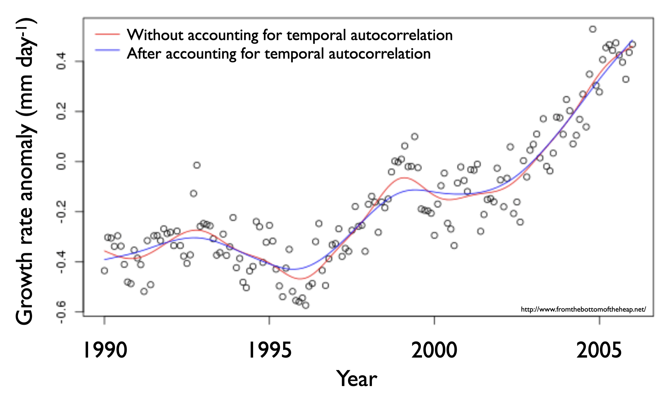
Suppose you want to test the hypothesis that variability in growth rate of newly hatched cod (torsk) in the Kattegat is explained by prey availability (Growth ~ Prey). The observations you are using to test this hypothesis have been collected over ~15 years, and it is likely that measurements made closer to each other in time are more similar than those made further apart from each other in time. This may be because the physical or biological environment was more similar in years that are close to each other in time (e.g. the parent population was similar, the temperature was similar). However, there is nothing in your hypothesis (Growth ~ Prey) to let R know which observations are close to each other in time. Thus, you violate the assumption of observation independence.
When a model is fit to data and the observations are dependent on their sampling time, similar values closer in time are given too much weight on the model coefficients and the model fit is biased (compare lines in the plot on the right).
How you know if you have a problem with temporal autocorrelation
You can find out if observation dependence due to temporal autocorrelation is influencing your model by plotting your model residuals vs. time. If you have a problem with observation dependence, there will be a pattern in your residuals when plotted against the offending variable - in this case time.
You can also determine how large the problem of temporal autocorrelation is by estimating the autocorrelation function24 and the Durbin-Watson test. An easy way to test the latter is with the testTemporalAutocorrelation() function in the DHARMa package.
What you do if your observations are influenced by temporal autocorrelation
As above, the assumption of observation independence means that your observations are independent of one another in all ways except for the predictors included in your hypothesis. We need to tell R about this temporal dependence in your model. This can be done by including time as a predictor in your model. Note that time will need to be a fixed effect as it is continuous, and will need to be modelled with a non-linear shape assumption25 to deal with the complicated form of the temporal autocorrelation.
Alternatively, you can tell R about the correlation structure of the data directly (i.e. how similarity in observations changes as observations are further and further away from each other).
Spatial autocorrelation
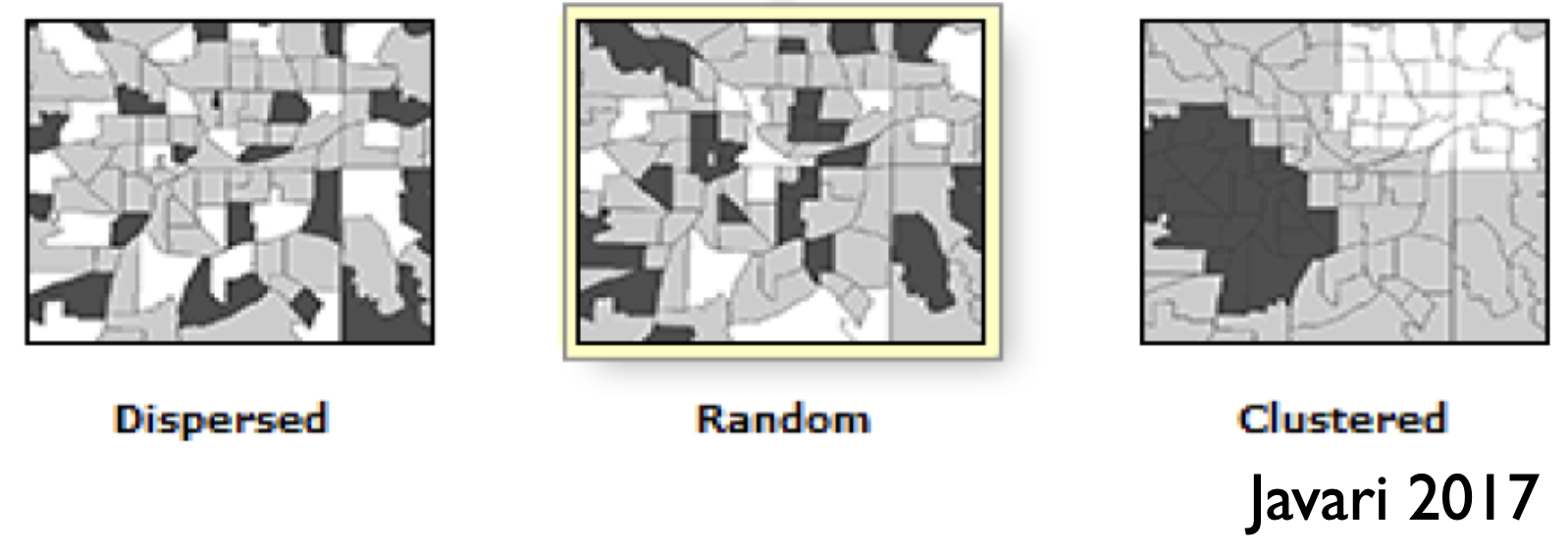
Similar to the previous section, spatial autocorrelation describes the dependence among observations that are collected at different spatial locations. Observations measured close to each other in space are more (or less!) likely to be similar to one another than those measured further apart. In the plot on the right you can see examples of observation dependence on space in the dispersed and clustered drawings. In the dispersed example, observations closer to each other in space are less likely to resemble each other than one would expect if observations were distributed randomly in space (random example). In the clustered example, observations closer to each other in space are more likely to resemble each other than one would expect if observations were distributed randomly in space.
An example
For example, you might be interested in how abundance of a species changes with mean environmental temperature and intend on testing the hypothesis that Abundance ~ Temperature. Measuring abundance over a large spatial area, you find that observations made closer to each other in space are more similar than those measured farther apart and part of this is due to effects other than temperature (e.g. other aspects of the environment such as food availability are more similar to each other for sites that are closer together). Without telling R information about where in space the observations were collected (remember, the hypothesis only includes Temperature), you violate the assumption of observation independence.
How you know if you have a problem with spatial autocorrelation
You can find out if observation dependence due to spatial autocorrelation is influencing your modelling by plotting your model residuals vs. location. As location is measured in two dimensions, you could try a bubble plot26 or variogram27 to help you look for patterns in your residuals with space. You can also estimate how big the problem of spatial autocorrelation is with Moran’s I test. The last can be done with the testSpatialAutocorrelation() function in the DHARMa package.
What you do if your observations are influenced by spatial autocorrelation
Similarly to our discussion about temporal autocorrelation, the location of the observations (e.g. latitude and longitude) can be included in your model to account for the spatial autocorrelation28. Alternatively, the dependence among observations due to proximity can be included in the model as a spatial autocorrelation structure.
A final point about observation independence
Remember that you only have to worry about your observations being dependent based on variables not already in your hypothesis.
6 Considering your error distribution assumption
What it is:
The error distribution (i.e. distribution of your residuals) needs to match the assumption29 you made when you chose your starting model. If this assumption is violated, the estimates of your coefficients will be less accurate, limiting your ability to use the model to test your hypothesis and make predictions.
How do you know if you have a problem:
You can compare the error distribution of your residuals with the distribution you expect given your error distribution assumption through something called a Q-Q plot. A Q-Q plot - or quantile-quantile plot - plots the two data distributions against each other via their quantiles30. When the expected and observed error distributions are in agreement, the points will fall along the red diagonal line in the Q-Q plot (the 1:1 line). You can also help your interpretation of this by null hypothesis goodness of fits tests (more on this below).
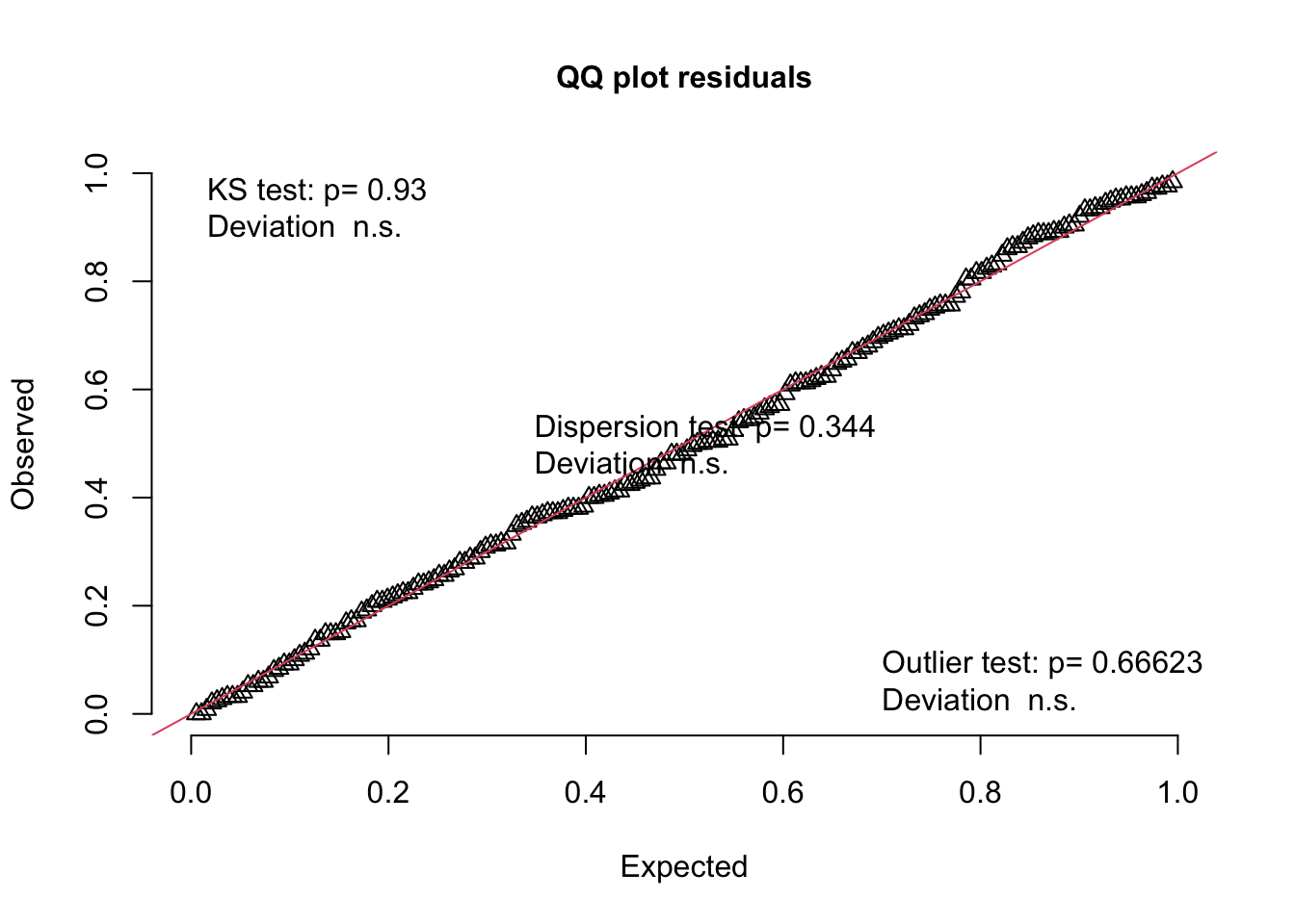
The scaled residuals method introduced above will allow you to consider the behaviour of your residuals in a similar way regardless of the structure of your model. You can get a Q-Q plot of your residuals with:
# Consider your error distribution assumption by inspecting observed vs. expected residuals:plotQQunif(simOut, # the object made when estimating the scaled residuals. See section 2.1 abovetestUniformity =TRUE, # testing the distribution of the residuals testOutliers =TRUE, # testing the presence of outlierstestDispersion =TRUE) # testing the dispersion of the distribution
Note that the plot is the observed vs. expected scaled residuals. As above, the triangular points will follow the red line in a well-specified model. You will generally assess this by eye, but the DHARMa package also includes three null hypothesis tests that give you more information about the behaviour of your residuals relative to the expected behaviour. In all cases, a low P-value (traditionally P < 0.05) means that there is evidence that the null hypothesis can be rejected (and your error distribution assumption is not valid).31
The tests are:
KS test: The Kolmogorov-Smirnov test tests the null hypothesis that the distribution of your residuals is similar to the expected distribution (here, a uniform distribution). A low P-value means there is evidence that the observed residuals are different than expected, and your error distribution assumption is not valid. You can also access this test directly with the testUniformity() function in the DHARMa package.
Dispersion test: This Dispersion test tests the null hypothesis that the dispersion of your residuals is similar to the expected dispersion. A low P-value means there is evidence that the observed dispersion is different than expected, and that your error distribution assumption is not valid. You can also access this test directly with the testDispersion() function in the DHARMa package.
Outlier test: This Outlier test tests the null hypothesis that the number of outliers in your observed residuals is similar to the expected number. A low P-value means there is evidence that you have outliers. You can also access this test directly with the testOutliers() function in the DHARMa package. You can also find the position (row number) of the outliers with the outliers() function (also in the DHARMa package). A general definition of an outlier is a value that is surprising relative to the majority of the data sampled (Venables and Ripley 2002). Just what is surprising will vary with the type of data distribution (e.g. the interquartile range) and functions in the DHARMa package look for values outside the range simulated when estimating the scaled residuals. You can read more about the methods DHARMa uses in the help files.
What to do if it is a problem:.
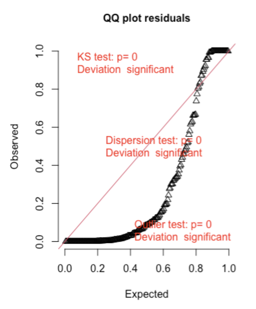
Here are two examples (from the DHARMA package vignette) of Q-Q plots where the error distribution assumption is not met:
First, here is an example of overdispersion, where there are too many residuals in the tails of the distribution and not enough in the middle of the distribution when compared to the expected:32
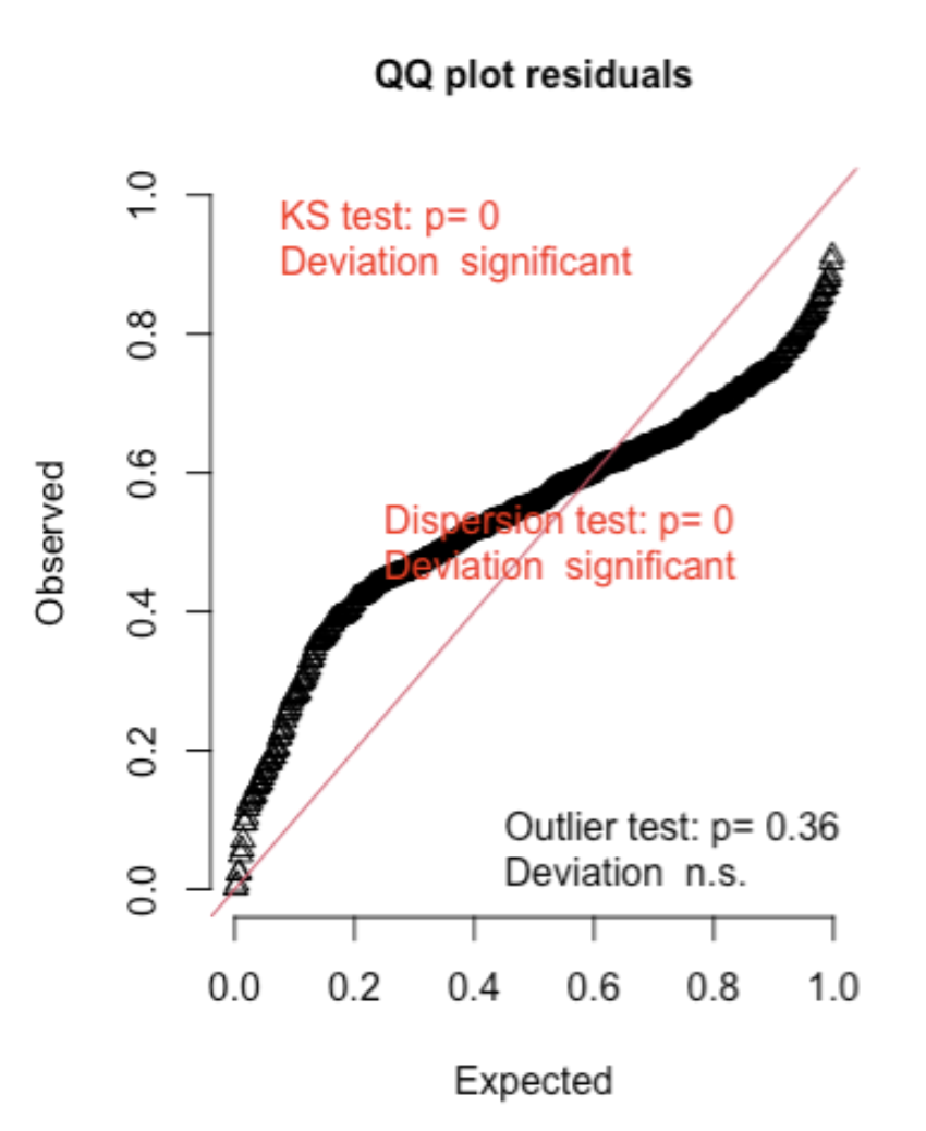
Second, here is an example of underdispersion, where there are too many residuals in the middle of the distribution and not enough in the tails of the distribution when compared to the expected:
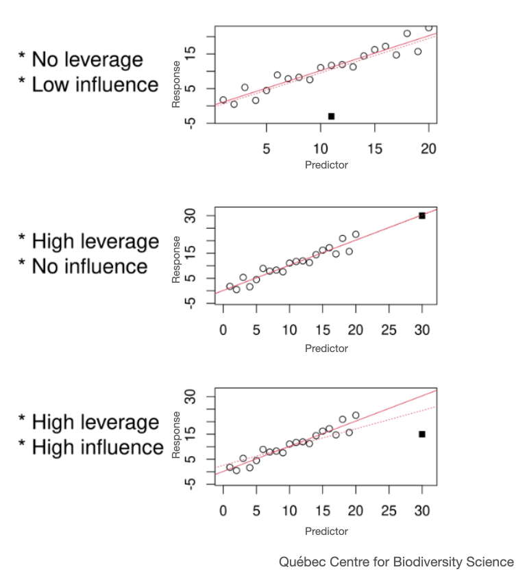
If your model residuals are not behaving as expected, you should first address any outlier problems. Explore the observations labelled as outliers and see if they should be kept in your data set. Outliers can be described in terms of their leverage and influence. A high leverage data point inflates the strength (certainty) of your modelled effects. This may or may not be classified as an outlier but should be explored for how it is influencing the strength of your modelled effects. On the other hand, an influential data point changes the estimate of your model effects (coefficients like slope and intercept) and may reduce the strength of your modelled effects.
Once you have explored outliers, if you still have residuals not behaving as expected, you can change your error distribution assumption and refit your starting model. This may mean you change the link function you used to fit the model. The link function we have been using is always the default link function - which you can see at the help file with ?family, but there are alternative link functions which can be used to help models that appear mis-specified. Try searching for alternative link functions online to get you started.
Alternatively, you can try changing the actual assumption (e.g. trying a normal distribution instead of a Gamma distribution). Note that with some types of response data (e.g. continuous) you have a number of different error distribution assumptions you can try (e.g. Gamma vs. normal), while others (e.g. binomial, presence/absence, etc.) are more limited.
Trying alternate error distribution assumptions
We focus here on four error distribution assumptions that are useful for biology: gaussian (normal), Gamma, poisson and binomial. Being aware that there are others will help you find your way in future hypothesis testing adventures.
For example, a negative binomial assumption can help for models where a poisson error distribution assumption is not enough as the negative binomial distribution includes an extra parameter that can help control data that is not quite following a poisson distribution (e.g. excess variance).
In all cases, you will refit your model with the new assumption choice and re-validate that new model, as described here. There will be times where you have tried everything and you still have evidence that your model is mis-specified. In these cases, look at the magnitude of the violation.
If the violation appears minor (e.g. only a minor pattern in your residuals), your model may still be useable. In such cases communicate the issue in your model validation assessment along with your attempts to correct it, and proceed with your hypothesis testing with a cautious eye.
If the violation appears major, you may need to move on to another method (e.g. random forest or Bayesian design) that can help you design a more customized model to test your hypothesis.
7 Considering your shape assumption
What it is:
You made an assumption about the shape of the relationship between your response and each predictor (e.g. a linear shape assumption). You need to make sure that the assumption you made was useful before you can have the confidence in the coefficient estimates you will use to test your hypothesis.
How do you know if you have a problem:
For this assumption, you need to look at how your residuals are scattered around your model fit. If your model is a useful one (“well-specified”), the scatter of those residuals will be even and uniform around the fit (“a uniform cloud”). You can inspect your residuals in this way by plotting the residuals vs. the fitted values.
Here is code for this using the DHARMa package:
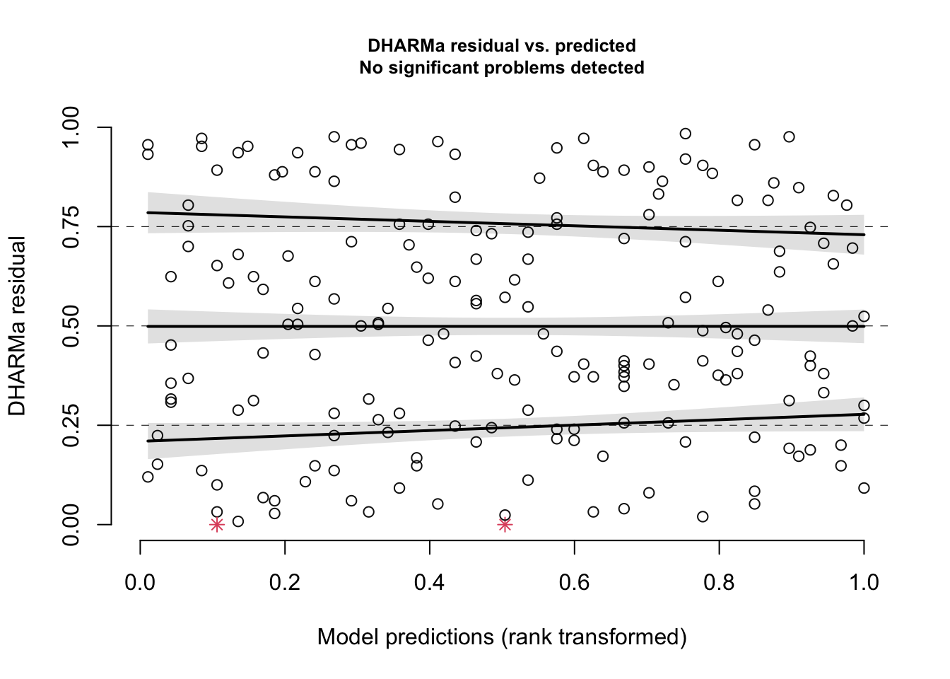
plotResiduals(simOut, # the object made when estimating the scaled residuals. See section 2.1 aboveform =NULL) # the variable against which to plot the residuals. When form = NULL, we see the residuals vs. fitted values
This gives a plot of the scaled residual (“DHARMa residual”) vs. the fitted values (“Model predictions”). Any simulation outliers (data points that are outside the range of simulated values, see also the section above) are highlighted as red stars. You can use the testOutliers() and outliers() function in the DHARMa package to learn more about outliers.
Again, you are looking for a uniform cloud of points. To help you assess the uniformity of the cloud, R adds quantile regression results: The three solid lines (called splines) are fit through the 0.25, 0.5 and 0.75 quantiles of the residual distribution. Quantile regression compares the empirical 0.25, 0.5 and 0.75 quantiles of the residuals (solid lines) with the theoretical 0.25, 0.5 and 0.75 quantiles (dashed line), These lines are then compared with a quantile test that tests the null hypothesis that these splines are not different than the dashed horizontal lines. If the null hypothesis of this is rejected, the curves will appear red in the figure, and you can determine your shape assumption was not valid.
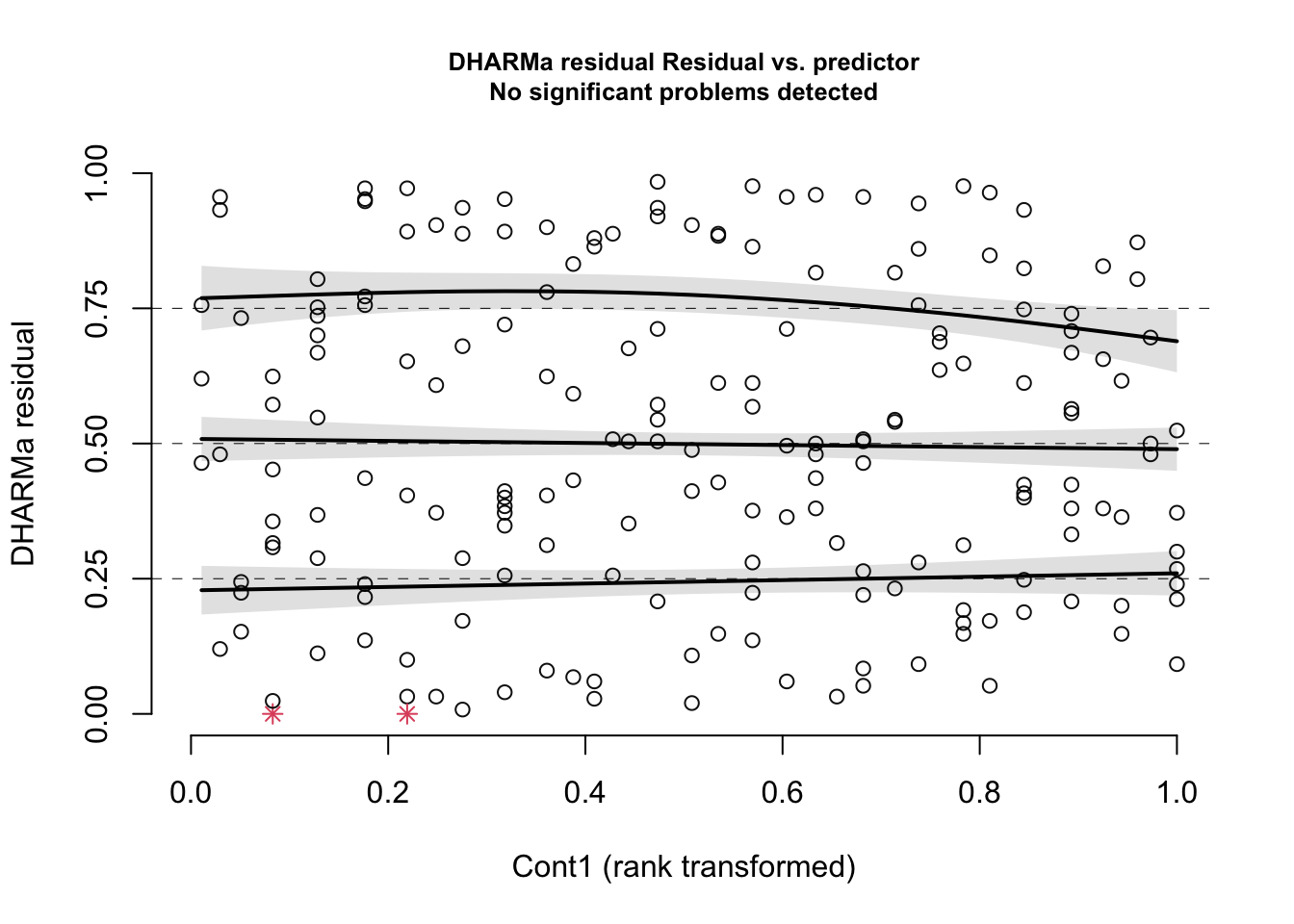
You should always inspect a plot of residuals vs. fitted values to explore your shape assumption. If you have multiple predictors in your model, you should also plot the residuals vs. each predictor to make sure the shape you chose for each relationship is useful. This will help to ensure that the shape assumption was correct for each of your predictor variables. Here are the residuals of our example model vs. the Cont1 predictor:
plotResiduals(simOut, # the object made when estimating the scaled residuals. See section 2.1 aboveform = myDat$Cont1) # the variable against which to plot the residuals. When form = NULL, we see the residuals vs. fitted values
and vs. the Cat predictor:
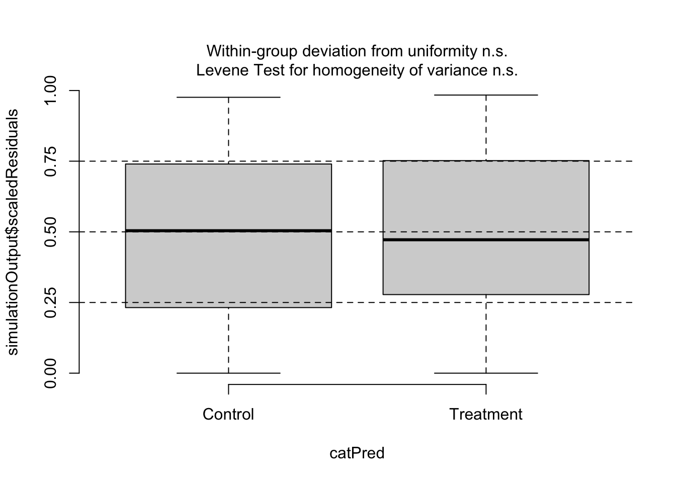
plotResiduals(simOut, # the object made when estimating the scaled residuals. See section 2.1 aboveform = myDat$Cat, # the variable against which to plot the residuals. When form = NULL, we see the residuals vs. fitted valuesasFactor =TRUE) # make sure R understands that this is a categorical predictor
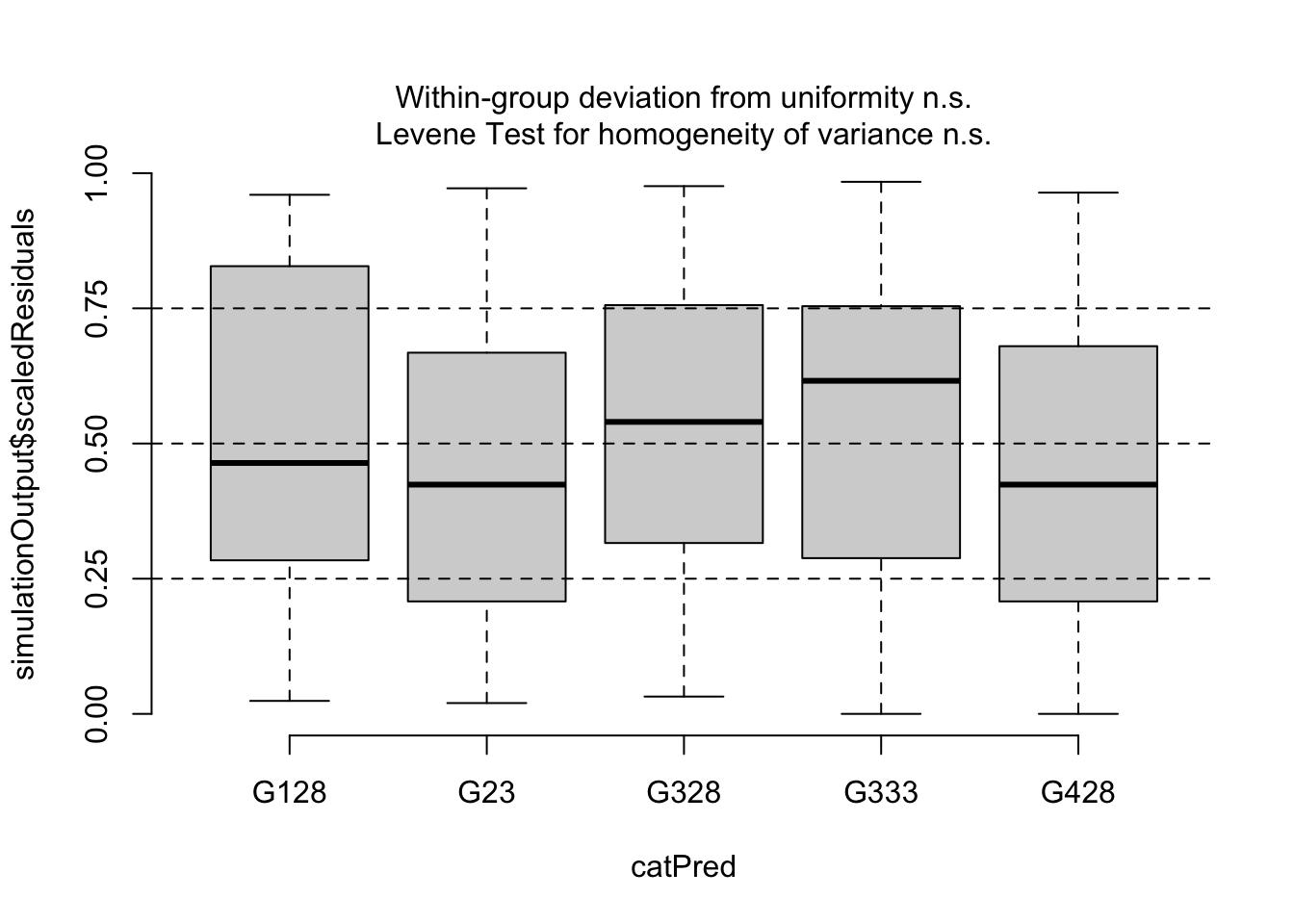
In this last figure, you get boxplots showing the distribution of the residuals - one for each level of your categorical predictor. This different picture is because the predictor Cat is categorical. Instead of a uniform cloud, you look for boxplots that spread across the 0.25 and 0.75 quantiles. If the spread is wide and even across the levels of your categorical predictor, you have evidence the model is well-specified to test your hypothesis. DHARMa also includes a Levene Test that tests if the variance across the levels in your categorical predictor are similar. If they are different, the Levene Test will be flagged in red with a p-value < 0.05.
Finally, you also want to plot your residuals with any predictor you left out of your model. This will help determine if it should be in your model (i.e. can explain variability in your response).
What to do if it is a problem:
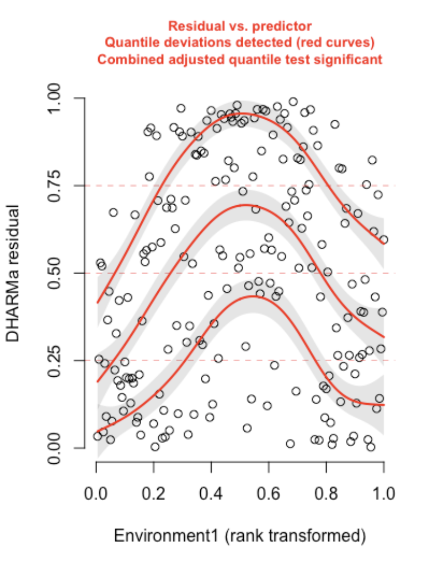
Here is an example of a residual plot when you have a violation in your shape assumption33:
In this case, the predictor Environment1 was fit with an assumption of a linear relationship with the response, when a non-linear shape assumption was needed. Note that you can also access the quantile test used to flag shape assumption violations with the testQuantiles() function in the DHARMa package.
If you find a pattern in your residuals that indicates a violation of your shape assumption, you can change your assumption and refit your model. This may mean changing the shape of the model (e.g. from linear to non-linear) and/or including an interaction in your model.34 You will refit your model with the new assumption choice and re-validate that the model is useful following the steps in this section. Note that quantile tests are sensitive for very large data sets. You may have quantile regression results flagged for minor problems if you have a very large data set even though the model is still usable to test your hypothesis (Hartig 2024). In all cases communicate any issues in your model validation assessment along with your attempts to correct it. Keep any remaining (minor) problems in mind as you proceed with your hypothesis testing with a cautious eye.
8 Summary - things to try when you have a problem with your residuals:
Summarizing from the sections above, here are your next steps if your residuals indicate that your model will have trouble testing your hypothesis:
Inspect any outliers in your data
Try modelling with a different link function
Try modelling with a different error distribution assumption
Is a potential predictor missing from your model?
Try a non-linear shape assumption
In all cases, report the process and results of your model validation
9 A final thought
As you can see, validating your starting model will sometimes lead you to make changes to your starting model that require you to refit your starting model and re-validate the new model It can feel a bit like you are walking in circles, but rest assured that this is very normal. And necessary: you can not go further to test your hypothesis until you are confident you have a useful model.
10 Up next
In the next section, we will discuss how you can use your validated model to test your hypothesis. Finally: the science!
Fox, John, and Georges Monette. 1992. “Generalized Collinearity Diagnostics.”Journal of the American Statistical Association 87 (417): 178–83. https://doi.org/10.1080/01621459.1992.10475190.
Porter, Lorenzo Ciannelli, Steven M., and Lew J. Haldorson. n.d. “Environmental Factors Influencing Larval Walleye Pollock Theragra Chalcogramma Feeding in Alaskan Waters.”Marine Ecology Progress Series 302: 207–17.
remember, these are the modelled effects of your predictors on your response↩︎
your predictors are so correlated, in fact, we say they are “aliased” with one another↩︎
the error (variance) around the coefficient estimates is getting bigger (inflated)↩︎
VIF can also be defined as the inverse of tolerance or the amount of variability in a particular predictor not accounted for by variability in the other predictors (Hebbali olsrr package 2024)↩︎
Other options include centering or detrending the offending predictor(s), combining information from one or more offending predictor e.g. by regressing the two offending predictors against one another and using those residuals as your model predictor (see here for an example (Porter and Haldorson, n.d.)), or using multivariate analysis (see the coming section on multivariate analysis), or using more conservative methods of fitting your model (estimating your coefficients) with e.g. a ridge penalty↩︎
the model can not have interactions when estimating VIFs because an interaction term will always be correlated with the main effect predictor terms involved in the interaction.↩︎
in your own work, you will choose the predictor to remove based on your domain knowledge, study’s goals and particular situation↩︎
notice I say “can be defined as…”. This is because there are many different definitions of a residual that have been made to deal with different model structures. We are going to use a very useful one - the scaled residual - that will let you explore residuals for a wide range of models. More on this below!↩︎
similar to Bayesian p-values or parametric bootstrapping↩︎
you made an error distribution assumption to match how your response is distributed, but note that it is the distribution of the residuals that matters, and you can only check this AFTER your model is fit. This error distribution is also called the conditional distribution↩︎
A quantile defines a particular part of a data set, e.g. the 90% quantile indicates the value where 90% of the values are less than the 90% quantile value. See the section on Data Distributions for more↩︎
“Deviation n.s.” on the plot means that there is no significant deviation from expected↩︎
Note that zero-inflated data (more zeroes than expected) appears similarly↩︎